

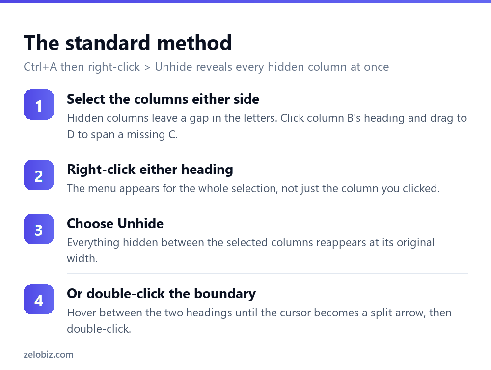
To unhide columns in Excel, select the columns on either side of the gap — the letters skip, so click B and drag to D to reveal a missing C — then right-click and choose Unhide. To reveal everything at once, press Ctrl+A then right-click any column heading and choose Unhide. Column A is different: there’s nothing to its left, so type A1 in the Name Box, press Enter, then use Home › Format › Hide & Unhide › Unhide Columns.
The Reason the “Reliable” Keyboard Shortcut Often Isn’t
Nearly every guide to unhiding columns lists Ctrl+Shift+0 as the fast, reliable keyboard method, right alongside the standard right-click menu approach. What almost none of them mention is that this specific shortcut is notoriously unreliable on real-world keyboards, for reasons that have nothing to do with anything you’re doing wrong in Excel.
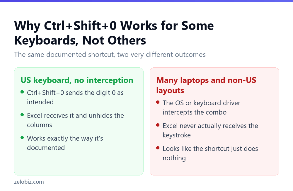
This is well known enough among long-time Excel users that it has its own small reputation, and it’s the reason experienced spreadsheet users tend to reach for the right-click Unhide method by default rather than the keyboard shortcut, treating Ctrl+Shift+0 as a nice-to-have rather than something to depend on.
⚠️ Watch out: There’s no universal, one-click fix inside Excel itself for a shortcut being intercepted somewhere else in the system, since that interception happens well before Excel is even involved in the process. The right-click method covered above, or Alt, H, O, U, L pressed as a sequence rather than held together, both route around the problem entirely and work regardless of what your specific keyboard or layout does with Ctrl+Shift+0.
Spotting what’s actually missing
Excel gives you two visual clues that a column is hidden, and both are subtle enough to miss on a busy sheet.
The obvious one is the letters skip — A, B, D, E means C is hidden. The second is a slightly thicker line between the two headings either side of the gap. On a zoomed-out sheet neither jumps out.
Before assuming something is hidden, check the sequence. People often conclude columns are hidden when the sheet is simply scrolled sideways, or when frozen panes are holding the first few columns in place while the rest moves.
Unhide everything at once
On an inherited spreadsheet with several gaps, going one at a time is slow. Ctrl+A selects the entire sheet, and right-clicking any column heading then choosing Unhide reveals every hidden column simultaneously.
Press Ctrl+A twice if the first press only selects the current data region rather than the whole sheet — Excel expands the selection each time you press it.
Same approach works for rows: Ctrl+A, then right-click any row number and choose Unhide. Do both and you’ve got the complete sheet back in about four seconds.
💡 Pro tip: Keyboard shortcuts if you prefer: Ctrl+Shift+0 unhides columns and Ctrl+Shift+9 unhides rows. The column one is disabled by default in some Windows language configurations, which is why it sometimes appears not to work.
Column A, and why the usual method fails
A specific, common frustration. Column A is hidden, and there’s no column to its left to include in a selection — so there’s nothing to span and Unhide is greyed out or does nothing.
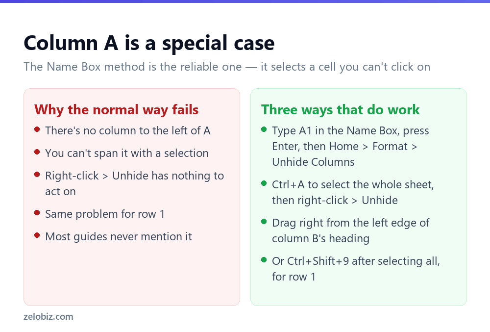
The Name Box is the reliable route. It’s the small box to the left of the formula bar showing the current cell reference. Type A1 into it and press Enter — you’re now inside the hidden column, even though you can’t see it. Then go to Home › Format › Hide & Unhide › Unhide Columns.
The dragging method also works if you have a steady hand. Move to the very left edge of column B’s heading until the cursor becomes a double-headed arrow with a split down the middle, then drag right. Column A reappears at whatever width you drag to, which is usually why people prefer the Name Box — you keep the original width.
Row 1 has exactly the same problem and exactly the same solution.
When unhide does nothing at all
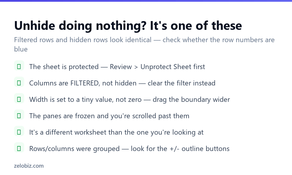
You select across the gap, click Unhide, and the columns stay missing. At that point they’re almost certainly not hidden — something else is going on.
The sheet is protected
If the worksheet is protected and ‘Format columns’ wasn’t allowed, Unhide is disabled. You’ll usually notice the option greyed out. Go to Review › Unprotect Sheet first — you may need the password.
It’s a filter, not hidden columns
This is the most common false alarm, and it applies mainly to rows. Filtered-out rows and hidden rows look identical, but Unhide won’t touch filtered ones.
The tell is the colour of the row numbers: filtered rows leave the remaining numbers blue rather than black, and the column with the filter shows a small funnel icon instead of a plain arrow. Clear it with Data › Clear, or Data › Filter to switch filtering off entirely.
The column is very narrow, not hidden
Someone can drag a column to a width of 0.1 rather than actually hiding it. The letter sequence stays complete — no gap — but nothing is visible. Unhide has no effect because nothing is hidden.
Select the columns either side, then Home › Format › Column Width and set an explicit value like 10. Or double-click the boundary to autofit.
Grouped columns
Grouping collapses columns behind a small + button in a bar above the headings. It looks like hiding and behaves differently. Click the + to expand, or use Data › Ungroup to remove the grouping entirely.
Hiding columns in the first place
The reverse operation, briefly, since it’s the same menu: select the columns, right-click, choose Hide. Or Ctrl+0 for columns and Ctrl+9 for rows.
For anything you’ll hide and show repeatedly — a working column, a set of monthly figures — grouping is better than hiding. Select the columns and press Shift+Alt+Right arrow, and you get a collapse button. Anyone opening the sheet can see there’s something collapsed and expand it, rather than not knowing it exists.
⚠️ Watch out: Hidden columns still hold data, and it still leaves the building. Sending a spreadsheet with a hidden ‘internal margin’ column means sending that column. Delete anything confidential rather than hiding it before sharing a file externally.
Finding out what’s hidden
Before sending a workbook, it’s worth checking what’s tucked away — particularly on a file you didn’t build.
File › Info › Check for Issues › Inspect Document runs the Document Inspector, which reports hidden rows and columns, hidden worksheets, comments and personal information in the file’s properties. It offers to remove them too, though take a copy first — removal is not reversible.
It’s the quickest way to answer ‘is there anything in here I don’t want to send’, and most people have never opened it.
Unhiding on a Mac and in Excel for the web
The menus differ slightly and it trips people moving between platforms.
On Mac, right-click and Unhide works the same, but the keyboard shortcuts don’t — use Ctrl+Shift+0 rather than the Command key, since Excel keeps the Windows binding here. The Name Box trick for column A is identical.
In Excel for the web, right-click and Unhide is available, but there is no Format menu under Home in older builds, so the column A workaround is the Name Box route only. Very hidden sheets can’t be revealed at all online — that needs the desktop app and the VBA editor.
Very hidden sheets
Worth knowing if a whole worksheet seems to be missing rather than a column. Excel has a third state beyond visible and hidden, called very hidden, which doesn’t appear in the right-click Unhide list at all.
Right-clicking a tab and choosing Unhide shows only normally hidden sheets. A very hidden one is invisible from the interface entirely, and can only be revealed through the VBA editor: press Alt+F11, find the sheet in the Project pane, and change its Visible property from xlSheetVeryHidden to xlSheetVisible.
It’s usually used by template authors to keep calculation sheets out of the way rather than to conceal anything. But if a workbook’s numbers come from somewhere you can’t find, this is where to look.
Everything above about Ctrl+Shift+0 applies equally to Ctrl+Shift+9, the equivalent shortcut for unhiding rows. It’s the same key combination pattern, so it’s intercepted by the same operating systems and keyboard drivers for the same reasons, and the same right-click or Alt-key workarounds apply without any changes. If one of the two shortcuts is unreliable on a particular machine, it’s worth assuming the other one probably is too, rather than testing each separately and hoping one behaves differently.
One specific, common cause is worth naming: Windows uses Ctrl+Shift plus a number or letter as a built-in shortcut for switching between installed keyboard layouts or input languages, on machines set up with more than one language installed. If a second keyboard layout was ever added, even briefly, that system-level shortcut can quietly claim the combination before Excel gets a chance to. Checking Settings, Time & Language, Language & region, for more than one keyboard listed under any language is a quick way to confirm whether this specific cause applies to a given machine.
Removing the extra keyboard layout, or reassigning the language-switching shortcut to something other than Ctrl+Shift plus a number, frees up Ctrl+Shift+0 for Excel to receive again. Neither change is required, and plenty of people work in more than one language and never touch this setting. It’s simply useful to know that fixing an unreliable Excel shortcut sometimes means adjusting a Windows setting that has nothing to do with Excel at all.
- ✓Check whether the letters actually skip before assuming
- ✓Use Ctrl+A then Unhide to clear a whole sheet at once
- ✓Use the Name Box for column A and row 1
- ✓Check for blue row numbers — that’s a filter, not hiding
- ✓Run Document Inspector before sending a file externally
- ✕Assuming Unhide is broken when the sheet is protected
- ✕Confusing filtered rows with hidden rows
- ✕Hiding confidential data instead of deleting it before sharing
- ✕Dragging column A open and losing its original width
- ✕Overlooking grouped columns behind a + button
Worked example: three ways to unhide the same column, in order of reliability
A shared workbook has column D hidden, and it needs to come back quickly for a report that’s due in about ten minutes. Here’s the order worth trying, most reliable first, rather than the order most tutorials happen to list them in.
Selecting C:E means clicking column C’s header, holding Shift, and clicking column E’s header, which selects all three columns including the hidden D in the middle even though you can’t click on D directly. Right-clicking anywhere in that selection and choosing Unhide brings it back immediately, and this works on every version of Excel on every keyboard, since it never depends on a key combination reaching the app correctly.
The Alt-key sequence is the other dependable option, and it’s worth learning even though it looks clunkier than a single shortcut. Press Alt, release it, then press H, then O, then U, then L in sequence, each one narrowing down through the ribbon: Home tab, Format menu, Hide and Unhide, Unhide Columns. It’s slower to type than Ctrl+Shift+0 but it goes through Excel’s own menu system rather than relying on a raw key combination, so nothing outside Excel gets a chance to intercept it.
Ctrl+Shift+0 stays useful as a first try since it’s genuinely fast when it works, which is most of the time on a standard US keyboard with no conflicting software running. Treat it as a shortcut worth attempting, not one worth depending on for something time-sensitive.
Frequently asked questions
Why doesn’t Ctrl+Shift+0 unhide columns on my computer?
On many laptops and non-US keyboard layouts, that key combination gets intercepted by the operating system or keyboard driver before it reaches Excel. Select the columns on either side of the hidden one and right-click Unhide instead, or use the Alt, H, O, U, L key sequence, both of which work regardless of keyboard.
How do I unhide all columns in Excel?
Press Ctrl+A to select the whole sheet, then right-click any column heading and choose Unhide. Do the same on a row number to unhide rows. Ctrl+Shift+0 is the keyboard shortcut for columns.
How do I unhide column A?
The normal method fails because there’s no column to its left. Type A1 in the Name Box beside the formula bar, press Enter, then use Home, Format, Hide & Unhide, Unhide Columns.
Why is Unhide not working in Excel?
Usually the sheet is protected, or the rows are filtered rather than hidden, or the column is set to a very small width rather than hidden. Check for blue row numbers, which indicate a filter, and try Review, Unprotect Sheet.
What’s the difference between hidden and filtered rows?
Hidden rows were deliberately hidden and are revealed with Unhide. Filtered rows are excluded by a filter and only come back when you clear it. Filtered sheets show the remaining row numbers in blue and a funnel icon on the filtered column.
Do hidden columns still contain data?
Yes. Hiding is purely visual — the data is still in the file and still travels with it when shared. Delete confidential columns rather than hiding them before sending a workbook externally.
Why can’t I see a worksheet even after choosing Unhide?
It may be set to ‘very hidden’, a state that doesn’t appear in the Unhide list. Press Alt+F11 to open the VBA editor, select the sheet, and change its Visible property to xlSheetVisible.
- →Clean up what you just revealed — how to remove duplicates in Excel
- →Lay out headings without breaking sorting: how to merge cells in Excel
- →Stop people changing your structure — how to lock cells in Excel
- →Pull data across sheets: how to use VLOOKUP