How to Freeze Rows in Excel (Pick the Right Cell First)

The rule that makes it make sense

Freeze Panes seems unpredictable until you know what it’s reading, and then it never surprises you again.

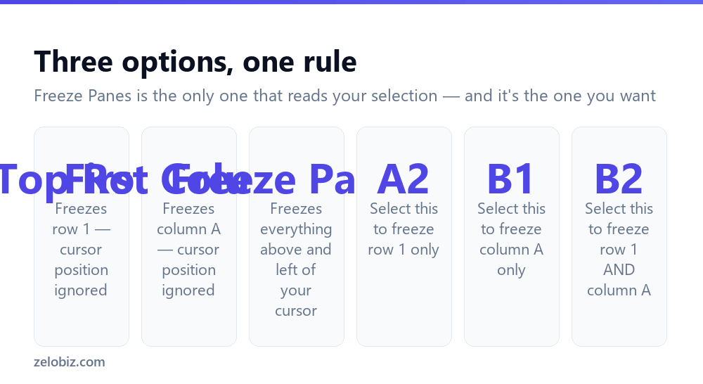
It freezes everything above and to the left of the selected cell. That’s the entire behaviour. The cell you have selected when you click the button determines the split, and nothing else does.

So to keep row 1 visible, select A2 — row 1 is above it. To keep column A visible, select B1. To keep both, select B2. To keep three header rows and two label columns, select C4.

The two shortcuts, and their limits

Freeze Top Row and Freeze First Column ignore your cursor completely and do exactly what they say. They’re convenient and they handle the two most common cases.

What they can’t do is freeze more than one row, more than one column, or both at once. For any of that you need the main Freeze Panes option and the cell-selection rule above.

They also can’t be combined. Clicking Freeze Top Row and then Freeze First Column doesn’t give you both — the second replaces the first. Excel supports exactly one frozen region per sheet.

Freezing rows and columns together

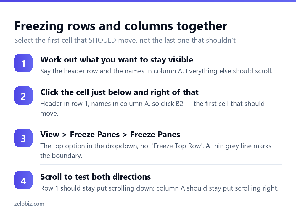
This is the setup that makes a wide table genuinely usable — headers stay across the top, identifying labels stay down the left, and the numbers scroll underneath.

A thin grey line appears at the boundary once it’s applied. If you see two lines, one horizontal and one vertical, you’ve frozen in both directions. One line means only one direction took effect, which usually means you selected a cell in row 1 or column A.

Undoing and changing it

The Freeze Panes button becomes Unfreeze Panes once something is frozen. There’s no way to adjust an existing freeze — you unfreeze, select the correct cell, and freeze again.

That’s the fix for the most common complaint, which is having frozen the wrong rows. Nothing is broken; the selection was just one cell out. Unfreeze, click the right cell, and reapply.

When the option is greyed out

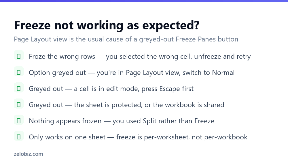
Page Layout view is the usual reason. Freeze Panes only works in Normal view — switch back via View › Normal or the small icons at the bottom-right of the window, and the option becomes available again.

Edit mode is the other. If you’re part-way through typing in a cell, most ribbon commands grey out. Press Escape and try again.

Protection or sharing can also block it, depending on how the workbook was set up. Check Review › Unprotect Sheet, and if the file uses the older shared-workbook feature, freezing is disabled entirely.

Freeze versus Split

Sitting next to Freeze Panes in the View tab is Split, which looks similar and behaves quite differently. People reach for one expecting the other.

Use Freeze when you want context that never moves. Use Split when you want to look at two distant parts of the same sheet simultaneously — the top pane can sit on row 5 while the bottom shows row 500, and both scroll independently.

You can’t have both active at once. Turning on Split removes an existing freeze, and vice versa.

What freezing doesn’t affect

Freeze Panes is purely a screen behaviour, and that catches people out in two places.

Printing ignores it entirely. A frozen header row does not repeat on page two of a printout. For that you need Page Layout › Print Titles › Rows to repeat at top, which is a separate setting that happens to do the printed equivalent. Setting one does not set the other.

It has no effect on formulas, sorting or filtering. A frozen row is still an ordinary row — it will be included in a sort if it falls inside the range, which is a reason to make sure your header row is properly recognised as a header rather than relying on it being frozen.

Keyboard shortcut and the ribbon route

There’s no single dedicated key, but the Alt sequence is quick once learnt: press Alt, W, F, F in order — not together. That’s View, Freeze Panes, Freeze Panes. Alt, W, F, R freezes the top row and Alt, W, F, C freezes the first column.

Pressing the same sequence again unfreezes, because the menu item toggles. Worth committing to memory if you open a lot of exported spreadsheets, where freezing the header is usually the first thing you do.

On a Mac the ribbon path is identical but the Alt sequences don’t apply. Use the View tab directly, or add Freeze Panes to the Quick Access Toolbar so it’s one click from any tab.

Very wide sheets and the disappearing frozen area

One genuine limitation: the frozen region has to fit on screen alongside something to scroll. Freeze twelve columns on a laptop display and there’s almost no room left for the data, which makes the sheet less usable rather than more.

Excel doesn’t prevent this. It will happily freeze more than fits, and the result is a window where the scrollable area is a narrow strip on the right. If scrolling suddenly feels broken after freezing, this is usually why.

Keep the frozen area to what genuinely provides context — typically one or two header rows and one identifying column. If you need more than that visible at once, the sheet is probably too wide and would be better split or pivoted.

Tables freeze headers automatically

If your data is an Excel Table — created with Ctrl+T — you may not need Freeze Panes at all.

Scroll down inside a Table and the column letters at the top of the sheet are replaced by the Table’s own headers. They stay visible without any freezing, and the filter arrows come with them.

Two caveats. It only applies while your cursor is inside the Table, and it replaces the column letters rather than sitting below them, which occasionally confuses people using cell references. For a sheet with several tables or a lot of surrounding content, an explicit freeze is still clearer.

Frequently asked questions