

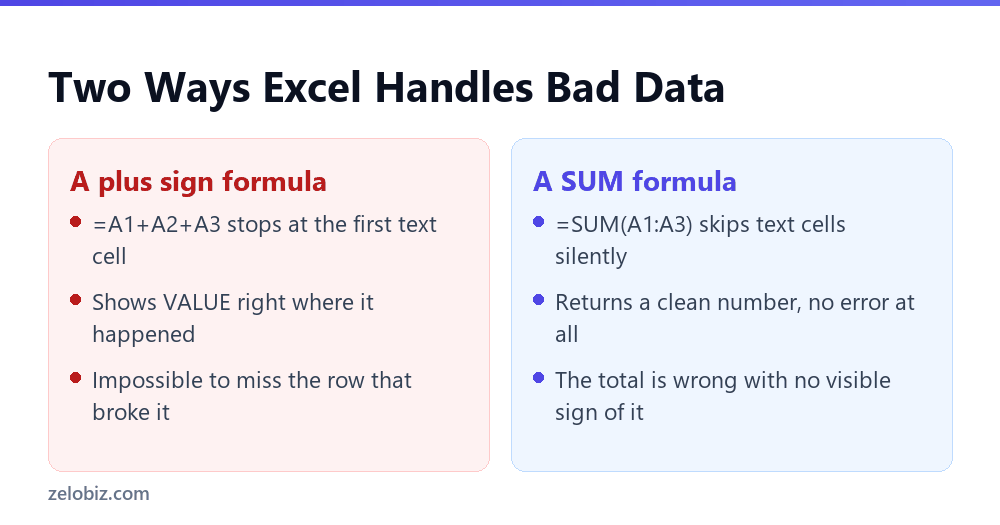
So a VALUE error shows up the moment a formula tries to do math on a cell holding text instead of a number. So it is loud, it is red, and it stops the whole formula cold.
So the standard fix is switching operators to a function. So replace =A1+A2+A3 with =SUM(A1:A3), and the error disappears. Problem solved, most guides say.
But it did not fix the bad data. So SUM just skips over text cells instead of erroring on them, and the total it returns is wrong, with nothing on screen to say so.
Switching a broken formula from plus signs to SUM does not fix a VALUE error, it avoids it. A plus sign formula like A1+A2+A3 stops and shows VALUE the moment it hits a text cell. SUM, AVERAGE, and similar functions instead skip any text cell entirely and calculate only from the numbers that remain, returning a clean result with no warning that anything was excluded. The fix removes the visible error, not the underlying data problem, so the total can be wrong in a way nobody notices. Verified against Microsoft’s own documentation on 18 September 2026.
What Actually Triggers a VALUE Error
So a VALUE error means a formula tried arithmetic on something that is not a number. So that covers more cases than it first looks like.
So the obvious case is a cell holding actual text, a word typed where a number belongs. But a number stored as text looks identical on screen and causes the exact same error, since Excel treats it as text underneath.
Also, a hidden character can cause this too. A number copied from a website often carries a non-breaking space, invisible in the cell, that quietly turns a real number into text as far as a plus sign formula is concerned.
The Fix Everyone Recommends
So switching to SUM is common advice, and it works, in the sense that the red error goes away. So that is exactly the problem.
So this distinction matters more than it sounds. A VALUE error is annoying, but it is honest. So it tells you exactly where the problem is. A quiet SUM total tells you nothing at all.
Where This Silently Breaks a Total
So say a monthly expense tracker sums ten rows of receipts in column B, using =SUM(B2:B11).
Then one receipt amount got pasted from an email as text, with a trailing space nobody can see. So SUM quietly excludes that one cell and adds the other nine, returning a number that looks completely normal.
⚠️ Watch out: Nothing about the result signals the problem. The total is simply short by whatever that one receipt was worth, and it will stay that way until someone happens to add the column up by hand and notices the gap.
So with a plus sign formula instead, that same sheet would show VALUE right where the bad cell sits, impossible to miss during any review.
Finding What SUM Is Actually Skipping

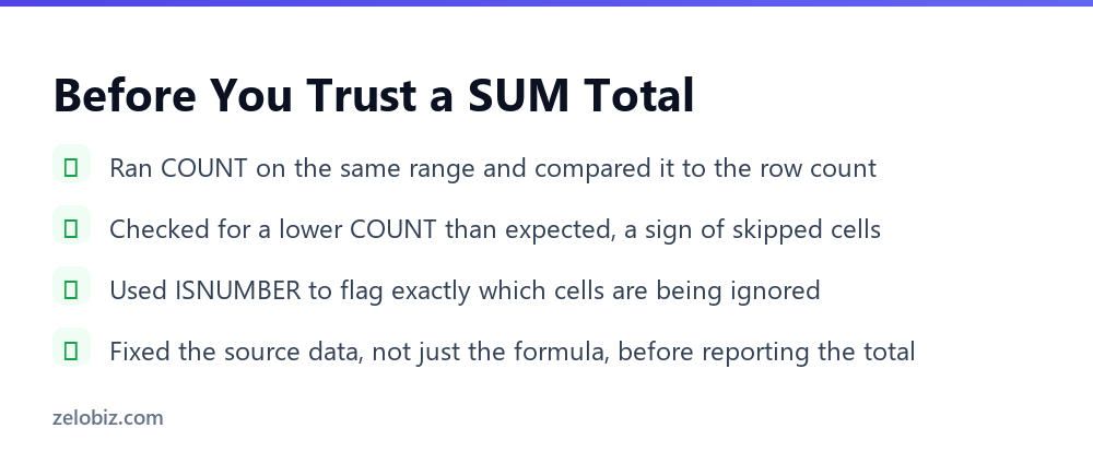
So the fix starts with a comparison, not a formula change. So run COUNT on the same range SUM is using, and compare it to the number of rows that should hold a number.
So if COUNT returns less than expected, some cells are not being read as numbers, even if they look like numbers on screen. So that gap is exactly what SUM has been quietly leaving out.
💡 Pro tip: Add a helper column with =ISNUMBER(A2) next to the range in question, then filter for FALSE. That flags precisely which cells are the problem, instead of scanning the whole column by eye.
A Worked Example
So a small business tracks weekly sales across five reps in a shared sheet, totaling each rep’s numbers with SUM at the bottom of their column.
One rep pastes their numbers from a text message screenshot converted to a spreadsheet, and three of the fifteen entries carry a hidden non-breaking space from that conversion. So SUM quietly drops those three from the weekly total.
Then the manager reviews the weekly totals and nothing looks wrong, since every column shows a plausible number. So the shortfall only surfaces a month later, during a quarterly reconciliation against actual bank deposits.
Running COUNT next to that rep’s column, back when the weekly total was first built, would have shown 12 instead of 15 immediately, catching the gap the same week it happened.
When the VALUE Error Is More Useful Than Silence
- →On a sheet still being built or checked, keep the plus sign formula so a VALUE error surfaces problems immediately.
- →Switch to SUM only once the data has been verified clean, not as the first response to an error.
- →Pair any SUM total with a COUNT check during setup, then drop the check once the sheet is trusted.
- →Treat a VALUE error as useful information, not just an annoyance to route around.
Cleaning Up the Actual Data
So once ISNUMBER flags the problem cells, the fix depends on what is actually wrong. So check the character first, then the format.
For a hidden non-breaking space, wrap the value in =VALUE(SUBSTITUTE(A2,CHAR(160),””)) to strip it and convert the result back to a real number. For an ordinary number stored as text, Data, Text to Columns, with no changes to the settings, often converts a whole column at once.
So either fix changes the actual cell, not just the formula reading it. That is the real difference between fixing the data and just working around it.
Preventing This on New Sheets
So most of this is preventable with one habit, built in from the start of any sheet that pulls data from outside Excel, like a website, an email, or a text export.
- →Add a COUNT check next to any SUM total while the sheet is still new.
- →Watch for a COUNT lower than the expected row count, the first sign something is being skipped.
- →Use ISNUMBER to flag the exact cells causing the gap, rather than guessing.
- →Convert pasted data with Text to Columns before trusting a total built on top of it.
Does This Apply to AVERAGE Too?
So yes, and arguably it is worse there. AVERAGE skips text cells the same way SUM does, but it also divides by fewer numbers than the row count suggests, since the excluded cells are not counted in the denominator either.
So a five row range with one text cell does not average across five numbers with a zero substituted in. So it averages across four, quietly changing the actual math, not just the total.
⚠️ Watch out: This can nudge an average in either direction depending on what the missing values would have been, and there is no way to tell from the result alone which way it moved or by how much.
Testing Whether Your Own Sheet Has This Problem
So a two minute check reveals whether a specific SUM total on your own sheet is trustworthy. So add =COUNT(range) next to the existing total.
Then compare that number to how many rows should hold data. If they match, the total is reading every cell as expected. So if they do not, the difference is exactly how many cells are being silently excluded right now.
💡 Pro tip: Run this check on any sheet where data arrives from outside Excel regularly, a form, an export, a copy and paste from email. Those are the sheets most likely to carry the hidden characters that cause this.
What About SUMIF and SUMIFS?
So SUMIF and SUMIFS behave the same way as plain SUM once a condition matches. So they skip a text cell in the sum range silently. The condition check itself does not change that.
So a report built on SUMIFS across a dozen categories can have this problem hiding in any one of them, and each category would need its own COUNT check to confirm nothing is being quietly excluded.
💡 Pro tip: On a sheet with several SUMIF or SUMIFS formulas, build one shared helper column with ISNUMBER first, then reference it from every condition. That catches a bad cell once, instead of debugging each total separately when the numbers do not add up later.
Why This Is Worse on a Growing Sheet
So a five row sheet checked by eye rarely hides this problem for long. A two hundred row sheet, fed by a monthly export, is a different story entirely.
So each new export can introduce its own hidden characters, inconsistent with the last one. The source system exporting the data may change formatting without warning anyone downstream.
So a check that worked fine on last month’s export is not a guarantee the same formula handles this month’s export the same way. Rerunning the COUNT comparison after every import is worth the ten seconds it takes.
A Faster Habit for Any New Total
So build the habit once, and it applies to every sheet after this one. Add COUNT next to SUM from the start, not after a total looks suspicious.
So it costs one extra cell. It takes seconds to set up. And it turns a silent gap into a visible number, every single time, without needing to remember to check.
Then once a sheet has been running clean for a while, the check can move to a separate tab, out of the way, still there whenever something needs a second look.
💡 Pro tip: Name the helper cell something obvious, like Row Count Check, rather than leaving it unlabeled. So the next person looking at the sheet understands what it verifies without asking.
What This Looks Like on a Finance Sheet
So a finance team pulling numbers from three different systems into one master sheet faces this risk on every column, not just one.
Each source system formats numbers slightly differently. So one might export currency with a symbol attached, another with trailing whitespace, and a third as clean numbers. Three different systems, three different silent failure modes, all hiding behind the same SUM formula.
So a COUNT check on each imported column, run right after every import, catches all three failure modes with one simple comparison, long before the numbers reach a report anyone outside the team will see.
Common Questions
Does switching from plus signs to SUM fix a VALUE error?
It removes the visible error, but it does not fix the underlying data. SUM skips any text cell in its range instead of erroring on it, so the total can be wrong with no warning.
How do I find which cells SUM is silently skipping?
Run COUNT on the same range and compare it to the expected number of rows. If COUNT is lower, add a helper column with ISNUMBER to flag exactly which cells are being excluded.
Does AVERAGE have the same problem as SUM?
Yes, and it can be worse. AVERAGE both skips text cells and divides by fewer numbers than the row count suggests, changing the calculated average, not just the total.
What causes a number to be stored as text without anyone typing it that way?
Pasting from a website, an email, or an export often carries a number as text, sometimes with an invisible character like a non-breaking space, even though it displays normally in the cell.
Is a VALUE error actually useful, or just annoying?
It is useful. It shows exactly where a formula hit bad data, which is more than a silent SUM total tells you. Keeping a plus sign formula during setup surfaces problems immediately instead of hiding them.
How do I fix a number that Excel treats as text?
Use Data, Text to Columns with no changes to the default settings, which often converts a whole column at once. For a hidden non-breaking space specifically, wrap the value in VALUE and SUBSTITUTE to strip it first.
Do SUMIF and SUMIFS have the same silent skipping problem?
Yes. So once a row matches the condition, SUMIF and SUMIFS add it up the same way plain SUM does, skipping a text cell in the sum range without any warning that it happened.
Is it worth keeping the COUNT check permanently, or just during setup?
For a sheet fed by regular imports or pasted data, keep it permanently. So a source that behaved cleanly last month is not a guarantee it behaves the same way on the next import.
The Short Version
- →A VALUE error means a formula tried arithmetic on something that is not a number.
- →Switching to SUM removes the error by skipping the bad cell, not by fixing it.
- →A SUM total can be silently wrong with no visible sign of the problem.
- →COUNT next to a SUM total reveals whether any cells are being excluded.
- →AVERAGE has the same blind spot as SUM, and changes the actual calculation, not just the total.
So the plus sign formula was never the problem here. It was doing its job, flagging bad data the moment it found it.
So the real fix was always fixing the data, not the formula around it. A clean total that skipped something is worse than an ugly error that told you where to look.
So the next time a VALUE error shows up, resist the urge to route around it right away. Find the bad cell first. Fix it there. Then decide whether SUM is safe to use, instead of hoping it quietly makes the problem disappear on its own.