Excel’s FILTER Function: The #CALC! Mistake Nobody Explains

Excel’s FILTER function replaces a whole family of clunky array formulas with one clean line. It also produces two different-looking errors that get mixed up constantly, even though they mean completely different things.

This covers the exact syntax, what #CALC! and #SPILL! actually indicate, and which Excel versions can even use FILTER in the first place.

The Syntax

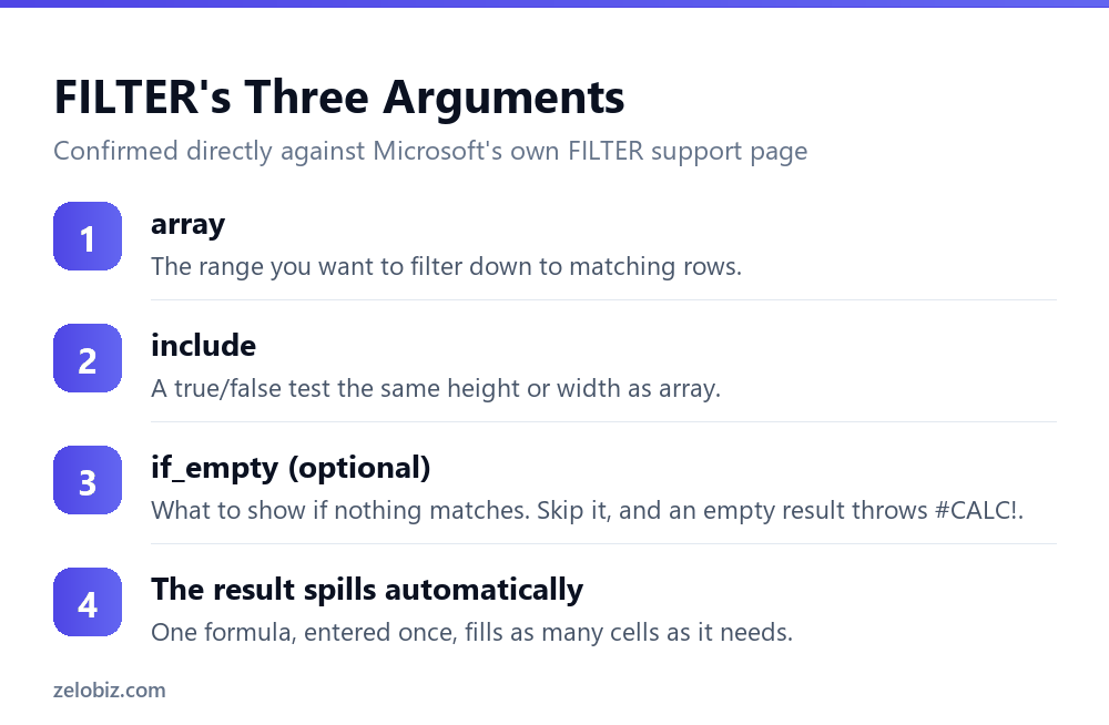
FILTER takes three arguments. The syntax is FILTER(array, include, [if_empty]).

A simple example: FILTER(A2:C100, B2:B100=”Active”) returns every row from A2:C100 where column B says Active. No helper columns, no array-entered formula, no Ctrl+Shift+Enter required.

So unlike older array formulas, FILTER just spills. Type it once, press Enter normally, and the result fills downward automatically into however many rows it needs.

What #CALC! Actually Means

So #CALC! shows up in one specific situation: the filter condition matched nothing at all, and there’s no fallback value telling Excel what to show instead.

Because FILTER needs to return something, an empty result with no if_empty argument is treated as an error rather than a blank cell. That’s a deliberate design choice, not a bug.

What #SPILL! Actually Means

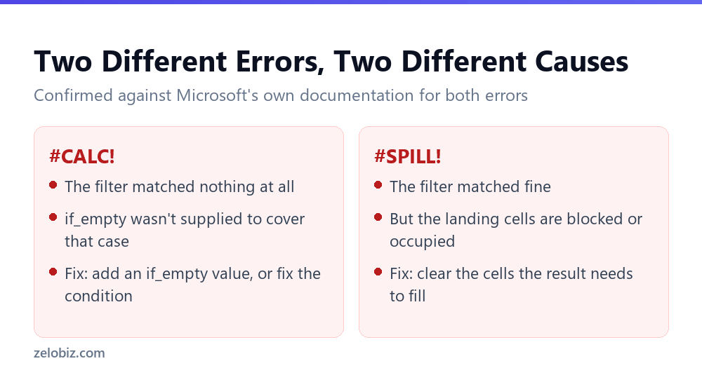
So #SPILL! is a completely different problem. It shows up when FILTER found real matches, but the cells below or beside the formula, where those results need to land, already contain something else.

That something else can be actual data, a merged cell, part of an Excel Table, or even hidden text. Any of them can physically block the spill range from filling.

Excel shows a dotted border around the space the result wanted to fill. That border is the fastest way to see exactly what’s in the way.

Where FILTER Actually Works

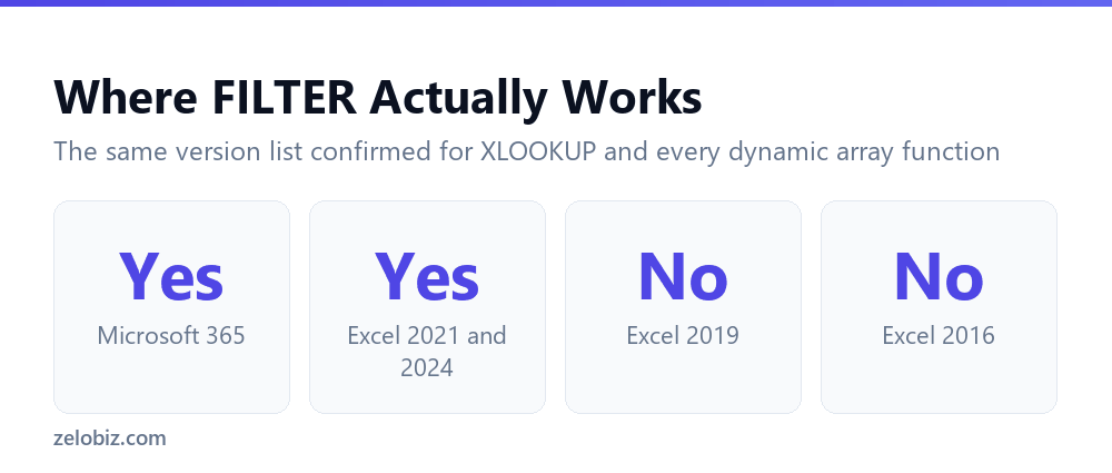
FILTER isn’t available everywhere. Microsoft’s own documentation lists Excel for Microsoft 365, Excel 2024, Excel 2021, and the mobile apps as supported. Excel 2019 and Excel 2016 are absent from that list entirely.

That’s the same version boundary as XLOOKUP and every other dynamic array function. So if your workplace runs a perpetual-license copy of Excel from that older window, FILTER simply isn’t there to use, regardless of how the formula is written.

A Practical Example, Start to Finish

So picture a task list in columns A through D, where column D marks each task’s status. A formula in F1 reads FILTER(A2:D200, D2:D200=”Overdue”, “Nothing overdue”).

When at least one task is marked Overdue, every matching row spills automatically below F1. Add a new overdue task anywhere in the source data, and the filtered list grows on its own the next time the sheet recalculates.

Clear every overdue flag, and the formula doesn’t error. It shows the text “Nothing overdue” instead, because the if_empty argument gave it something to fall back on.

But if someone types a value directly into F2, the cell FILTER’s first result row needs, the very next recalculation throws #SPILL!, since that cell is no longer empty and available.

FILTER vs. the Old Way

So before FILTER existed, getting the same result meant either Advanced Filter, a multi-step dialog buried on the Data tab, or a nested array formula using IF and SMALL together.

Both older approaches worked, but neither updated cleanly. Advanced Filter had to be re-run manually every time the source data changed. The nested array formula technically updated automatically, but it was dense enough that few people could read it back a year later.

FILTER replaces both. One readable formula, entered once, that recalculates and respills automatically whenever the source data changes. That’s the actual improvement, not just shorter syntax.

Combining FILTER With Other Functions

So FILTER doesn’t have to stand alone. Nesting it inside other functions extends what it can do considerably.

SORT(FILTER(range, condition)) filters first, then sorts the result, all in one formula. That combination alone replaces a lot of manual Data tab work.

COUNTA(FILTER(range, condition, “”)) counts how many rows matched, since COUNTA counts non-blank results. Wrapping FILTER inside a summary function like this is a common, practical pattern.

Multiple conditions work too, joined with the multiplication operator instead of AND: FILTER(range, (condition1)*(condition2)) returns rows where both conditions are true at once.

A Common Mistake With the include Argument

So one mistake shows up often enough to call out directly: mismatching the size of array and include.

If array covers rows 2 through 200, include has to cover the exact same range, row for row. A mismatch, even by a single row, produces a #VALUE! error rather than a silently wrong result.

Filtering on Multiple Columns With Different Logic

So real filtering needs often combine AND logic with OR logic in the same formula, not just one or the other. FILTER handles both, but the syntax looks different for each.

AND logic, where every condition must be true, uses multiplication: (B2:B100=”Active”)*(C2:C100>100). Both conditions have to hold for a row to make it through.

OR logic, where any one condition is enough, uses addition instead: (B2:B100=”Active”)+(B2:B100=”Pending”). Either condition being true keeps the row in the result.

So the operator, multiplication or addition, is what actually changes the logic here, not the structure of the formula around it.

Why FILTER Sometimes Feels Slower on Big Sheets

So on a very large dataset, tens of thousands of rows, FILTER can feel noticeably slower to recalculate than expected.

That’s usually because FILTER is set to scan whole-column references, like B:B instead of B2:B50000. A whole-column reference forces Excel to evaluate over a million rows even when the real data ends far earlier.

Switching to an exact range, or better, an Excel Table reference that grows automatically with the data, usually fixes the slowdown without losing the convenience of an auto-updating range.

What FILTER Doesn’t Do

So it’s worth being direct about the edges of what FILTER handles, since it’s easy to expect more from it than it actually delivers.

FILTER doesn’t sort its own results. Combine it with SORT if order matters, since FILTER alone preserves the original row order of whatever matched.

FILTER also can’t filter based on formatting, like cell color, only on actual values and formulas. A condition has to be something Excel can evaluate as true or false, not something purely visual.

Common Questions

The Short Version

Checking Your Excel Version Before Committing

So before building an entire workbook around FILTER, it’s worth spending ten seconds confirming it will actually work for everyone who needs to open the file.

Open File, then Account. If it lists Microsoft 365, Excel 2024, or Excel 2021, FILTER is available. Anything older, and the formula will show as an error or plain text the moment the file opens there.

For a workbook shared outside your own organization, this check matters even more, since there’s no way to control what version a recipient happens to be running.

A Habit Worth Building

So the broader habit worth taking from all of this: read the specific error code, not just the fact that something’s red.

#CALC! and #SPILL! look almost identical at a glance, both hash-prefixed, both appearing in place of the expected result. But they point in opposite directions, one toward the condition, one toward the destination cells.

Spending a few seconds identifying which error actually appeared saves far more time than guessing at a fix and checking whether it happened to work.

Nesting FILTER Inside a Chart or Pivot Table

So FILTER’s spilled output can feed directly into a chart, since a chart source range can simply point at the top-left cell of the spill and grow with it automatically as the underlying data changes.

That’s a genuinely useful pattern for a dashboard that needs to show, say, only overdue items or only this month’s entries, without rebuilding the chart’s source range every time the filter condition’s results change size.

Pivot tables work differently. A pivot table’s source range generally needs to be a stable range or an Excel Table, not a spilled array whose size changes. For a pivot-based summary, filtering the source data with a slicer or the pivot’s own field filters remains the more reliable approach than feeding it a FILTER result.

So keep FILTER and pivot tables as separate tools solving separate problems, rather than expecting one to fully replace the other across every kind of summary a workbook might need.