

VLOOKUP finds a value in the first column of a range and returns something from another column in the same row. The syntax is =VLOOKUP(what_to_find, where_to_look, which_column, FALSE). Two things cause most problems: it can only search the leftmost column of the range you give it, and if you leave off that final FALSE it defaults to approximate matching and will happily return the wrong answer.
What it actually does
You have an order list with product codes, and a separate price list. VLOOKUP is how you pull the price across without copying anything by hand.
=VLOOKUP(A2, Prices!A:C, 3, FALSE) reads as: take the code in A2, look for it down column A of the Prices sheet, and when you find it, return whatever’s in the third column of that range.
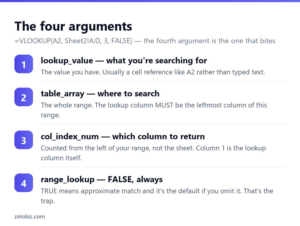
That distinction catches people constantly. col_index_num counts from the left edge of the range you specified, not from column A of the worksheet. If your range starts at column D, then column 1 is D, column 2 is E, and so on.
The fourth argument is not optional
Excel lets you omit range_lookup, and that’s the single worst design decision in the function.
Leave it out and Excel assumes TRUE — approximate match. It then assumes your data is sorted ascending, walks down until it passes the value it’s looking for, and returns the row before that. On unsorted data the result is essentially arbitrary.
Approximate match doesn’t error. It returns a plausible-looking wrong answer, which is considerably worse than #N/A.
Always type FALSE or 0 as the fourth argument. The only time TRUE is correct is banded lookups — tax brackets, commission tiers, grade boundaries — where you genuinely want ‘the largest value not exceeding this’, and your table is sorted ascending.
⚠️ Watch out: If a VLOOKUP is returning wrong values rather than errors, check the fourth argument before anything else. This is the most expensive Excel bug there is, precisely because nothing looks broken.
It can only look right
The lookup column must be the leftmost column of the range you pass in. VLOOKUP searches that column and returns something to its right. It cannot return anything to the left.
So if your product codes sit in column C and the names you want are in column A, VLOOKUP simply cannot do it. No argument changes that.
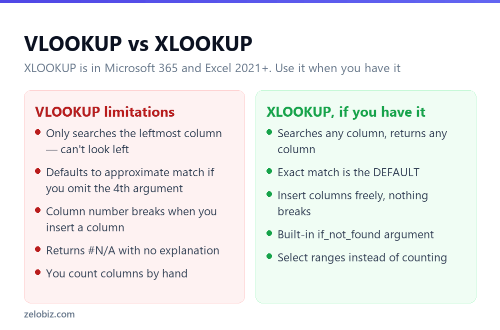
Three ways round it. Move the column so the lookup field is leftmost — crude but often fine. Use INDEX and MATCH together, which has no direction restriction: =INDEX(A:A, MATCH(F2, C:C, 0)). Or use XLOOKUP if your Excel has it, which handles either direction natively.
XLOOKUP, if you have it
Microsoft 365 and Excel 2021 onwards include XLOOKUP, which was written specifically to fix VLOOKUP’s problems.
=XLOOKUP(A2, Prices!A:A, Prices!C:C) — you give it what to find, the column to search, and the column to return. No counting, no leftmost restriction, and exact match is the default.
It also takes an optional fourth argument for what to show when nothing matches: =XLOOKUP(A2, Prices!A:A, Prices!C:C, "Not found"). That replaces the IFNA wrapper VLOOKUP needs.
Worth knowing VLOOKUP isn’t going anywhere — it’s in millions of spreadsheets and still works. But for anything new, XLOOKUP is simply better, and knowing both means you can read old workbooks and write better new ones.
Fixing #N/A
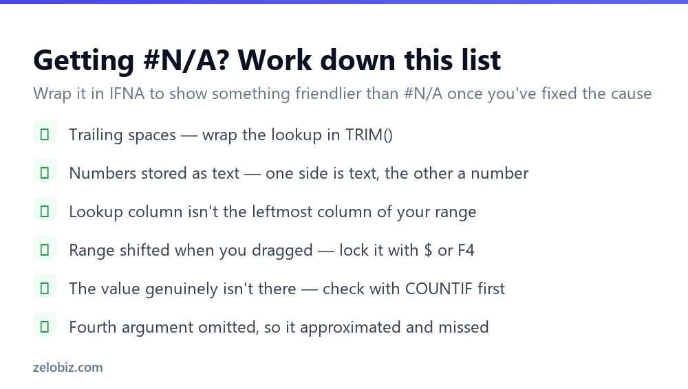
#N/A means ‘I looked and didn’t find it’. Usually the value is there and something invisible is preventing the match.
Trailing spaces
Data exported from another system frequently carries spaces you can’t see. "ABC123" and "ABC123 " are different values. Wrap the lookup in TRIM: =VLOOKUP(TRIM(A2), Prices!A:C, 3, FALSE).
If the spaces are in the lookup table rather than your search value, TRIM on the formula won’t help — you’ll need to clean that column first, or use a helper column of trimmed values.
Numbers stored as text
The other big one. Order number 1001 stored as a number will never match ‘1001’ stored as text, and both look identical on screen. The clue is alignment: text sits left in the cell, numbers sit right.
Fix the source column with Data › Text to Columns › Finish, which forces Excel to re-evaluate each value. Or coerce in the formula — =VLOOKUP(A2&"", ...) to make it text, or =VLOOKUP(VALUE(A2), ...) to make it a number.
The range moved when you dragged
Copy a VLOOKUP down a column and the range shifts down with it — row 10’s formula looks at a range starting nine rows lower, so it stops finding things partway down.
Lock it with dollar signs: $A$2:$C$500, or select the range and press F4 while editing. Using whole columns — A:C — sidesteps it entirely and is fine on modern Excel.
Making misses look tidy
Once you’ve established that some values genuinely aren’t in the table, wrap the formula so it shows something useful instead of #N/A.
=IFNA(VLOOKUP(A2, Prices!A:C, 3, FALSE), "Not found") displays your message when the lookup misses and the real value otherwise. IFERROR does the same but catches every error, which will hide genuine formula mistakes as well — IFNA is the more precise choice.
💡 Pro tip: Don’t reach for IFNA until you’ve worked out why the misses happen. Hiding #N/A before diagnosing it is how a spreadsheet ends up quietly missing a third of its data.
Making it survive column changes
col_index_num is a hard-coded number, so inserting a column into your lookup table silently changes which field gets returned. The formula doesn’t error — it just starts returning the wrong column.
Replace the number with a MATCH that finds the column by its heading: =VLOOKUP(A2, Prices!$A:$Z, MATCH("Price", Prices!$A$1:$Z$1, 0), FALSE). Now it looks for the column called Price wherever it happens to be, and inserting columns changes nothing.
It’s a longer formula, and worth it on anything other people will edit. The failure mode it prevents is silent and easy to miss for months.
Looking up on two conditions
VLOOKUP matches one value. Real questions are often ‘the price for this product in this region‘, which needs two.
The standard workaround is a helper column joining the fields into one key. In your lookup table add =A2&"|"&B2, and search for =VLOOKUP(F2&"|"&G2, ...). The pipe character stops false matches where values run together — without it, ‘AB’ + ‘123’ and ‘A’ + ‘B123’ both become ‘AB123’.
XLOOKUP handles it without a helper column by multiplying the conditions: =XLOOKUP(1, (A:A=F2)*(B:B=G2), C:C). Denser to read, but nothing extra to maintain.
When VLOOKUP is the wrong tool
Two cases where reaching for it is a mistake.
Combining large tables. Thousands of VLOOKUPs recalculating make a workbook crawl. Power Query’s Merge does the same job as a one-off operation with no live formulas — Data › Get Data, and it’s dramatically faster on big data.
Summarising rather than matching. If the question is ‘total sales per region’ rather than ‘the value for this specific key’, you want SUMIFS or a Pivot Table. VLOOKUP returns the first match it finds and ignores the rest, which quietly under-reports when keys repeat.
- ✓Always type FALSE as the fourth argument
- ✓Check the lookup column is leftmost in your range
- ✓Lock the range with $ or use whole columns
- ✓Use XLOOKUP for anything new if you have it
- ✓Diagnose #N/A before wrapping it in IFNA
- ✕Omitting the fourth argument and trusting the result
- ✕Assuming col_index_num counts from column A of the sheet
- ✕Hard-coding a column number in a sheet others will edit
- ✕Using VLOOKUP to total things — that’s SUMIFS
- ✕Hiding errors before you know what’s causing them
Frequently asked questions
What is the formula for VLOOKUP?
=VLOOKUP(lookup_value, table_array, col_index_num, FALSE). For example =VLOOKUP(A2, Prices!A:C, 3, FALSE) finds the value from A2 in column A of the Prices sheet and returns the third column of that range.
Why does VLOOKUP return #N/A?
The value wasn’t found. Most often that’s trailing spaces, numbers stored as text on one side, a lookup column that isn’t leftmost in your range, or a range that shifted when you copied the formula down.
Can VLOOKUP look to the left?
No. It only searches the leftmost column of the range and returns values to the right. Use INDEX and MATCH together, or XLOOKUP, if you need to return something to the left.
What does the FALSE at the end of VLOOKUP mean?
It requests an exact match. If you omit it, Excel defaults to TRUE — approximate match — which assumes sorted data and can return a wrong value without any error. Always include FALSE unless you specifically want banded matching.
Should I use VLOOKUP or XLOOKUP?
XLOOKUP if you have Microsoft 365 or Excel 2021 and later. It searches in any direction, defaults to exact match, doesn’t break when columns are inserted, and handles missing values directly. VLOOKUP remains useful for reading older workbooks.
How do I VLOOKUP with two conditions?
Add a helper column joining the fields, such as =A2&”|”&B2, and look up the joined value. Or in Microsoft 365 use =XLOOKUP(1, (A:A=F2)*(B:B=G2), C:C), which needs no helper column.
- →Clean the keys before matching — how to remove duplicates in Excel
- →Merged cells break lookups: how to merge cells in Excel
- →Protect the formulas once they work — how to lock cells in Excel
- →Find the lookup table someone hid: how to unhide columns in Excel