How to Add a Drop Down List in Excel That Updates Itself

The quick way, and what it costs

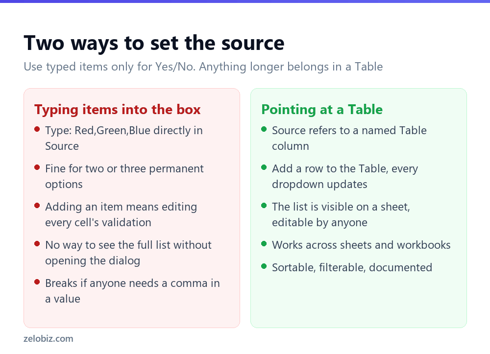
The two-minute version: select your cells, Data › Data Validation, Allow: List, and type Red,Green,Blue into Source. Click OK and you have a dropdown.

For a permanent two-option choice — Yes/No, Active/Inactive — that’s genuinely the right answer. Anything longer and you’ve created maintenance work for yourself, because the list now lives inside a dialog box that nobody else will think to look in.

The version that maintains itself

The upgrade is to keep your options on a worksheet, as a Table, and point the validation at it.

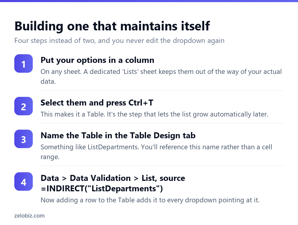
The reason Tables matter is that they grow. A plain range like =Lists!$A$2:$A$20 is fixed — type an option in A21 and no dropdown sees it. A Table expands automatically when you add a row underneath, and anything referencing it expands too.

In the Source box, use =INDIRECT("TableName[ColumnName]") — for example =INDIRECT("ListDepartments[Department]"). The INDIRECT wrapper is needed because Data Validation won’t accept a structured Table reference directly, which is an old Excel quirk rather than anything you’ve done wrong.

Letting people add their own options

A dropdown that rejects anything new becomes a bottleneck — someone needs a value, you’re not at your desk, and they type it into the notes column instead.

Two ways round it. Set the Error Alert to Warning rather than Stop, so people can override with a confirmation and you can review the odd entries later. Or leave a few blank rows at the bottom of the source Table and tell people to add there — with a Table source, anything they add appears in the dropdown immediately.

The second is usually better on a shared workbook. It keeps every value in one visible place rather than scattered through overridden cells, and the list stays usable for filtering and pivots afterwards.

Autocomplete and long lists

Excel dropdowns don’t have a search box. On a list of 200 customers, scrolling eight rows at a time is painful.

There’s a partial workaround: type the first few characters directly into the cell and Excel’s AutoComplete offers matching values it has seen elsewhere in that column. It works from existing entries in the column rather than from the validation list, so it improves as the sheet fills up.

For a genuine searchable dropdown you need a Combo Box from the Developer tab, or in Microsoft 365 a helper column using FILTER to narrow the source as someone types. Both are considerably more work — worth it for a form used daily, overkill for anything else.

Referencing another sheet

In current Excel you can point Source at another sheet directly: =Lists!$A$2:$A$20. In older versions that’s rejected, which is why so many guides tell you to use a named range.

To do it that way: select your options, type a name into the Name Box beside the formula bar, press Enter. Then in Source, type =YourName. Named ranges work from any sheet in any version.

They’re also easier to read six months later. =DepartmentList tells you what the dropdown contains; =Lists!$C$4:$C$19 tells you nothing.

Controlling what happens on a wrong entry

The Error Alert tab in Data Validation decides how strictly the list is enforced, and the default isn’t always what people expect.

If your dropdown feeds a VLOOKUP or a pivot, use Stop. A single free-typed value that doesn’t match your list produces #N/A downstream and takes far longer to find than it did to type.

Write something useful in the error message too. ‘The value you entered is not valid’ is the default and helps nobody; ‘Pick a department from the list, or ask Finance to add a new one’ actually resolves the situation.

Dependent dropdowns

The one people ask for most: pick a country in one cell, and the second dropdown shows only that country’s cities.

Set up one named range per parent option, each named exactly as the parent value — a range called France holding French cities, one called Spain holding Spanish ones. Then in the second dropdown’s Source, use =INDIRECT(A2), where A2 holds the first dropdown’s value.

INDIRECT converts the text ‘France’ into a reference to the range named France. It’s elegant and it’s fragile in one specific way: named ranges can’t contain spaces. ‘United Kingdom’ has to become United_Kingdom, and your parent list must match exactly, so most people use =INDIRECT(SUBSTITUTE(A2," ","_")) to handle it.

When the dropdown stops working

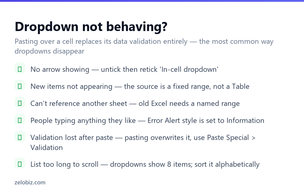
The arrow disappeared. Someone pasted a value over the cell. Pasting copies the source cell’s formatting and its validation — or lack of it — over the destination. Reapply the validation, and tell people to use Paste Special › Values instead.

New items aren’t showing. Your source is a fixed range rather than a Table. Convert it with Ctrl+T and update the Source to the INDIRECT form above.

The list is too long to use. Excel dropdowns display eight items at a time with a scrollbar, and there’s no setting to change that. Sort the source alphabetically so people can navigate by typing the first letter, which jumps down the list.

Removing or copying validation

To remove a dropdown: select the cells, Data › Data Validation, click Clear All, then OK. The cell keeps its current value and simply stops restricting future entries.

To apply the same dropdown elsewhere, copy a cell that already has it, then use Paste Special › Validation on the target. That copies the rule without the value or the formatting, which is usually exactly what you want.

To find every cell on a sheet that has validation: press F5, click Special, and choose Data validation. Useful when you’ve inherited a workbook and need to know where the rules are.

Frequently asked questions