

To use conditional formatting in Excel, select the cells you want to format, go to Home › Conditional Formatting, and choose a rule type — Highlight Cells Rules for simple comparisons, Data Bars or Color Scales for visualising a range of numbers, or Custom Formula for anything more specific. The formatting updates automatically whenever the underlying value changes — no manual re-colouring needed.
The rule types, and when to use each
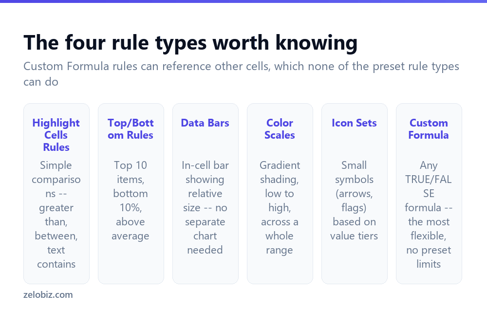
Highlight Cells Rules covers the basics — greater than, less than, between, equal to, text that contains a word, dates in a range, and duplicate values. This is the right starting point for most straightforward highlighting.
Top/Bottom Rules highlights relative standing rather than a fixed threshold — top 10 items, bottom 10%, above or below the average of the selected range. Useful when “which values matter” depends on the data itself, not a number you’d type in advance.
Data Bars draws an in-cell bar proportional to the value, giving a quick visual sense of relative size across a column without building a separate chart.
Color Scales shades every cell along a gradient from low to high (or a three-point low/mid/high scale), good for spotting patterns across a large grid of numbers at a glance.
Icon Sets places a small symbol — arrows, traffic-light circles, flags — next to each value based on which tier it falls into.
Custom Formula is the one preset rules can’t replace: it’s the only type that can compare a cell against a value somewhere else in the sheet, rather than a fixed number typed into the rule itself.
Applying a basic rule
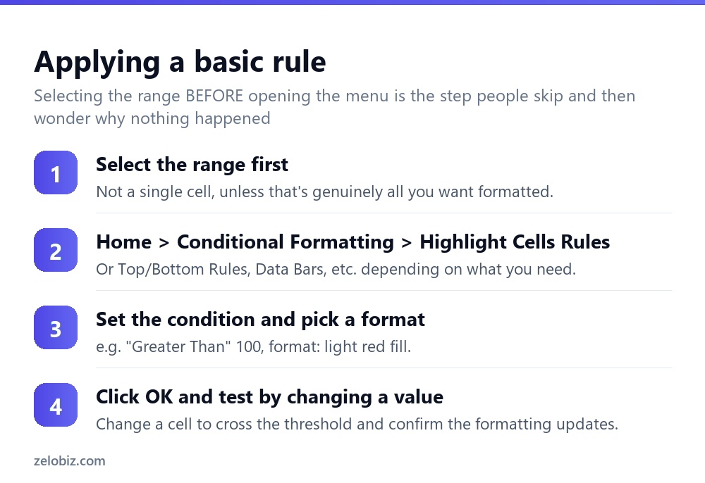
Select the range first — this is the step people skip, then wonder why nothing happens when they open the menu. Conditional formatting applies to whatever was selected at the moment you opened the dialog, not to the whole sheet.
Home › Conditional Formatting › Highlight Cells Rules › Greater Than (or whichever comparison fits). Type the threshold value, pick a format from the dropdown or click Custom Format for full control over fill colour, font colour, and border.
Click OK, then test it by changing a value in the range so it crosses the threshold — confirming the formatting actually updates is worth the ten seconds before moving on.
Custom Formula rules
This is where conditional formatting stops being a fixed-threshold tool and becomes genuinely flexible. Conditional Formatting › New Rule › Use a formula to determine which cells to format, then enter any formula that evaluates to TRUE or FALSE.
=B2>C2 highlights B2 whenever it’s greater than C2 in the same row — comparing two columns against each other, which none of the preset rule types can do. =WEEKDAY(B2)=1 highlights Sunday dates. =COUNTIF($A$2:$A$100,A2)>1 flags duplicates using your own logic rather than the built-in duplicate detector.
The formula is written relative to the first (top-left) cell of the selected range, and Excel adjusts it automatically for every other cell — exactly like a normal formula copied down a column.
Absolute vs relative references — the detail that breaks Custom Formula rules
This is the single most common source of a Custom Formula rule highlighting the wrong cells. If the rule should compare every row’s B against that same row’s C, use plain B2>C2 — relative, adjusts per row. But if the rule should compare every cell against one fixed cell — say, everything above a target stored in $F$1 — that reference needs dollar signs: B2>$F$1. Without them, Excel shifts F1 to F2, F3, and so on for each row, checking against a moving (and usually empty) target instead of the one fixed cell you meant.
💡 Pro tip: If a Custom Formula rule highlights an apparently random pattern of cells instead of what you expected, a missing dollar sign is the first thing to check.
Managing multiple rules
A range can carry more than one rule at once, and Conditional Formatting › Manage Rules shows all of them for the current selection, in the order they’re evaluated.
Order matters: rules are checked top to bottom, and a rule with Stop If True ticked prevents any rule below it from also applying to that cell. Without it, a cell matching two rules gets both formats applied, which can produce an unexpected result if the two formats conflict (one setting a fill colour, another overriding the font colour, for instance).
Use the up/down arrows in Manage Rules to reorder, and tick Stop If True on a rule whenever a lower-priority rule shouldn’t apply once a higher one has already matched.
Making a rule apply to new rows automatically
A rule applied to a fixed range like A2:A100 stops working the moment data extends past row 100 — new rows simply have no rule attached to them.
Two fixes: convert the range to an Excel Table (Ctrl+T) before applying the rule, since Table formatting extends automatically to new rows as they’re added; or apply the rule to a deliberately oversized range from the start (A2:A10000) so there’s headroom before it runs out, at the cost of the rule technically covering empty cells below your real data.
A worked example combining formats
Say a project tracker has a Due Date column (C) and a Status column (D). Two rules together give a useful at-a-glance view without touching either column’s raw values.
Rule 1 — overdue and not done: =AND(C2, format: red fill. This only fires when both conditions hold, which a single preset rule can’t express.
Rule 2 — due this week: =AND(C2>=TODAY(),C2<=TODAY()+7,D2<>"Complete"), format: yellow fill. Placed below Rule 1 in Manage Rules, with Rule 1’s Stop If True ticked, so an overdue row shows red only, never both colours competing.
Reading it back top to bottom in Manage Rules should tell the same story as the plain-English description — if it doesn’t, that’s usually a sign the rule order or a Stop If True checkbox needs adjusting.
Clearing rules without losing manual formatting
Conditional Formatting › Clear Rules › Clear Rules from Selected Cells (or Clear Rules from Entire Sheet) removes only the conditional rules, leaving any manually applied formatting — borders, a header row’s bold text, a deliberately coloured cell — exactly as it was. This is the safer option compared to selecting the range and clearing all formatting with the Format menu, which would strip manual formatting too.
When it’s not behaving
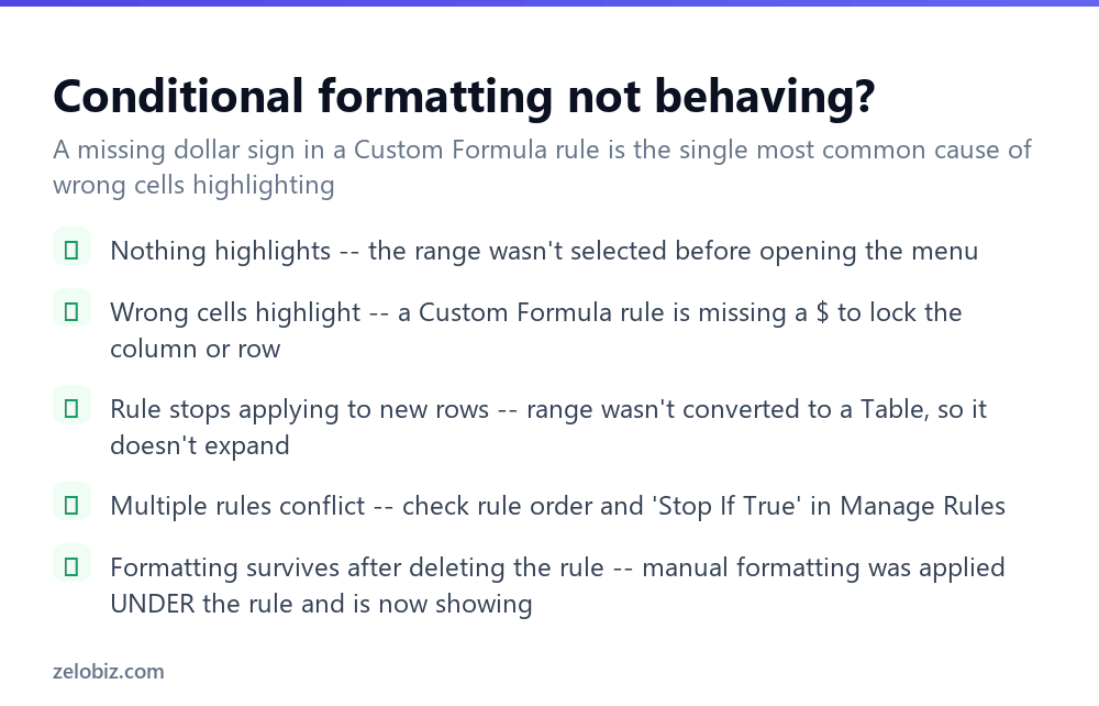
Nothing highlights at all — confirm the range was actually selected before the rule was created. Check Manage Rules and look at “Applies to” for the rule — if it only covers one cell instead of the intended range, that’s the fix.
Wrong cells highlight in a Custom Formula rule — almost always a missing dollar sign on a reference that should have stayed fixed. See the absolute-vs-relative section above.
Formatting survives after deleting the rule — conditional formatting sits on top of a cell’s regular manual formatting, not instead of it. If a cell was manually filled red before a conditional rule was ever added, removing the rule reveals that manual red fill underneath, which looks like the rule didn’t actually delete.
- ✓Select the range before opening the Conditional Formatting menu
- ✓Use dollar signs in Custom Formula rules referencing a fixed cell
- ✓Convert the range to a Table so new rows inherit the rule automatically
- ✓Tick Stop If True when a lower-priority rule shouldn’t also apply
- ✓Test a new rule by changing a value to confirm it actually updates
- ✕Applying a rule to a single cell by accident and wondering why nothing highlights elsewhere
- ✕Leaving out $ in a Custom Formula rule meant to reference one fixed cell
- ✕Applying a rule to a fixed range that data will eventually outgrow
- ✕Stacking conflicting rules with no Stop If True and getting an unpredictable result
- ✕Confusing manual cell formatting underneath a rule for the rule itself
Frequently asked questions
How do I apply conditional formatting in Excel?
Select the range, go to Home, Conditional Formatting, and choose a rule type such as Highlight Cells Rules, Data Bars, or Custom Formula.
What is a Custom Formula rule?
A conditional formatting rule based on any formula that returns TRUE or FALSE, which can compare a cell against another cell — something the preset rule types can’t do.
Why does my conditional formatting highlight the wrong cells?
Usually a missing dollar sign in a Custom Formula rule. A reference meant to stay fixed (like $F$1) shifts per row if the dollar signs are left out.
How do I make conditional formatting apply to new rows automatically?
Convert the range to an Excel Table with Ctrl+T before applying the rule — Table formatting extends to new rows automatically as they’re added.
Can I apply more than one conditional formatting rule to the same cells?
Yes. Rules are evaluated in the order shown in Manage Rules, and Stop If True prevents lower rules from also applying once a higher one matches.
Why does formatting stay after I delete a conditional formatting rule?
Conditional formatting sits on top of a cell’s manual formatting, not instead of it. Deleting the rule reveals whatever manual formatting was there underneath.
- →Test conditions with a formula first: how to use the IF function in Excel
- →Highlight budget overruns: how to make a budget in Excel
- →Total values that meet a condition: how to use SUMIF in Excel
- →Look up a value to format against: how to use INDEX MATCH in Excel