How to Use IF Function in Excel (With Real Examples)

The three arguments

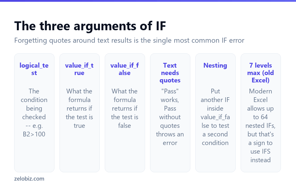
logical_test is any comparison that evaluates to TRUE or FALSE — B2>100, C2="Complete", D2<>"" (not blank), and so on. It’s the only genuinely required part of the syntax that has to be a real comparison.

value_if_true and value_if_false can be text (in quotes), a number, a cell reference, a calculation, or even another formula entirely. Leaving either one out isn’t an error — Excel returns TRUE or FALSE as the value for the argument you skipped, which is rarely what you actually wanted.

Writing your first one

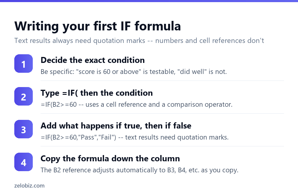
Start by stating the condition in plain language, specifically enough that it could be answered with a single comparison. “The score is 60 or above” is testable as B2>=60. “The student did well” isn’t testable at all until you decide what “well” means numerically.

Build the formula left to right: =IF(B2>=60,"Pass","Fail"). Text results go in quotation marks; the comparison itself doesn’t need any.

Copy the formula down the column and the B2 reference adjusts relatively to B3, B4, and so on — unless you’ve locked it with a dollar sign, which usually isn’t what you want for a row-by-row test like this one.

Common real-world patterns

• =IF(B2>=90,"A",IF(B2>=80,"B",IF(B2>=70,"C","F"))) — grade bands via nested IF
• =IF(D2="","Missing",D2) — show “Missing” for blank cells, the value otherwise
• =IF(C2>TODAY(),"Upcoming","Past") — compare against today’s date
• =IF(AND(B2>60,C2="Active"),"Eligible","Not eligible") — two conditions combined
• =IF(B2="","",B2*1.1) — calculate only if the cell isn’t blank, avoiding a 0 result

That last pattern is worth remembering on its own — it prevents a formula from showing a misleading calculated result (like 0) on rows that are simply empty and not yet filled in.

Combining IF with AND, OR, and NOT

IF’s logical_test can only directly hold one comparison, but wrapping it in AND, OR, or NOT lets it test several conditions at once.

=IF(AND(B2>60,C2="Active"),"Eligible","Not eligible") — both conditions inside AND must be true. =IF(OR(B2>90,C2="VIP"),"Priority","Standard") — either condition inside OR being true is enough. =IF(NOT(C2="Complete"),"Follow up","Done") — inverts a single condition, useful for “anything except X”.

AND and OR can each hold more than two conditions, separated by commas — AND(B2>0,B2<100,C2="Active") is a valid three-condition test.

Nested IF, and when to stop

Nesting an IF inside the value_if_false of another IF builds a chain of conditions, useful for grade bands, tiers, or ranges. Each level checks a narrower condition than the one before it, and the last value_if_false is the catch-all.

It works, but it stops being readable fast. Beyond three or four nested levels, most people (including the person who wrote it) lose track of which condition catches which value. Two better options at that point:

IFS (Excel 2019 and Microsoft 365) tests a list of conditions in order without nesting: =IFS(B2>=90,"A",B2>=80,"B",B2>=70,"C",TRUE,"F"). The final TRUE,"F" pair acts as the catch-all, equivalent to the last value_if_false in a nested chain.

A lookup table with VLOOKUP or INDEX MATCH is often clearer still for genuine range-based tiers -- store the breakpoints and labels in a small table, and look them up rather than hardcoding each threshold into the formula itself.

A worked example

Say column B holds a test score out of 100 for 40 students. A few real questions and the IF formula that answers each:

Simple pass/fail: =IF(B2>=60,"Pass","Fail"). One threshold, two outcomes.

Pass/fail with a note for borderline scores: =IF(B2>=60,"Pass",IF(B2>=55,"Borderline","Fail")). A second, nested IF catches the 55-59 range before falling through to Fail for anything lower.

A bonus that only applies to passing students: =IF(B2>=60,B2+5,B2) -- notice both branches here are calculations, not text, and neither needs quotation marks since they're numbers and cell references, not literal words.

Flag students needing a retest, but only if they were marked present: two conditions that must both be true calls for AND inside the test: =IF(AND(B2<60,C2="Present"),"Retest",""). Absent students with a low score get an empty result rather than an incorrect "Retest" flag.

Building formulas this way -- one specific question at a time, checked against a handful of rows you can verify by eye -- catches a backwards comparison or a missing quotation mark immediately, rather than after it's been copied down 40 rows.

IF with dates

Comparing dates inside an IF works the same as comparing numbers, since Excel stores dates internally as numbers -- but a few patterns come up often enough to note directly.

=IF(C2 compares a due date against today's date, recalculating automatically each day the file is opened. =IF(C2="","No Date Set",IF(C2 extends that to also catch rows where the date hasn't been entered yet, which otherwise would evaluate as 0 (Excel's earliest date) and incorrectly show as badly overdue.

Building an IF formula from a written rule

A useful habit for anything more complex than a single threshold: write the rule out in plain English first, as a nested series of if/then/otherwise statements, before touching Excel at all.

"If the score is 90 or above, grade A. Otherwise, if it's 80 or above, grade B. Otherwise, if it's 70 or above, grade C. Otherwise, grade F." Each "otherwise, if" becomes one nested IF, and translating line by line makes it far harder to lose track of a condition midway through, compared to writing the whole nested formula in one pass directly into a cell.

IF returning a formula result rather than text

Both branches of an IF can be calculations rather than fixed text or numbers -- =IF(B2>1000,B2*0.9,B2) applies a 10% discount only above a threshold, returning a calculated number either way rather than a label. This is a genuinely different pattern from the Pass/Fail examples above, and it's the one that trips people up when they assume IF can only ever return text.

IF versus IFERROR

These get confused because both start with IF, but they solve different problems. IF branches on a condition you define. IFERROR catches whatever error a different formula produces and substitutes a fallback value instead.

=IFERROR(VLOOKUP(A2,D:E,2,0),"Not found") shows "Not found" instead of #N/A when the lookup fails -- it isn't testing a condition you wrote, it's catching a formula error. The two are often combined: an IF for your own logic, wrapped in IFERROR to handle whatever might go wrong inside it.

When something's not working

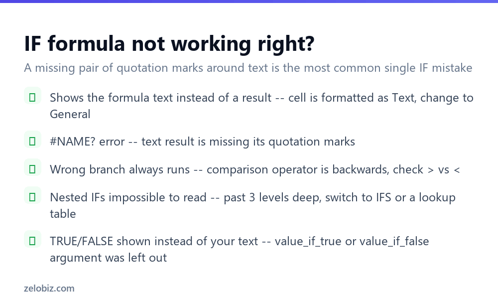
The cell shows the formula text itself, not a result -- the cell is formatted as Text rather than General or Number. Change the cell format, then re-enter the formula (a format change alone doesn't force recalculation of an existing formula).

#NAME? error -- almost always a text result missing its quotation marks. =IF(B2>60,Pass,Fail) fails because Excel reads Pass and Fail as names it doesn't recognise, not as text.

The wrong branch always runs -- check the comparison operator direction. B2>60 and B2<60 are easy to swap by accident, and Excel won't flag it as an error since both are valid comparisons.

TRUE or FALSE appears instead of your intended text -- one of the value_if_true or value_if_false arguments was left out entirely, and Excel filled in the test's own boolean result instead.

Frequently asked questions