How to Use INDEX MATCH in Excel (Instead of VLOOKUP)

What each function does on its own

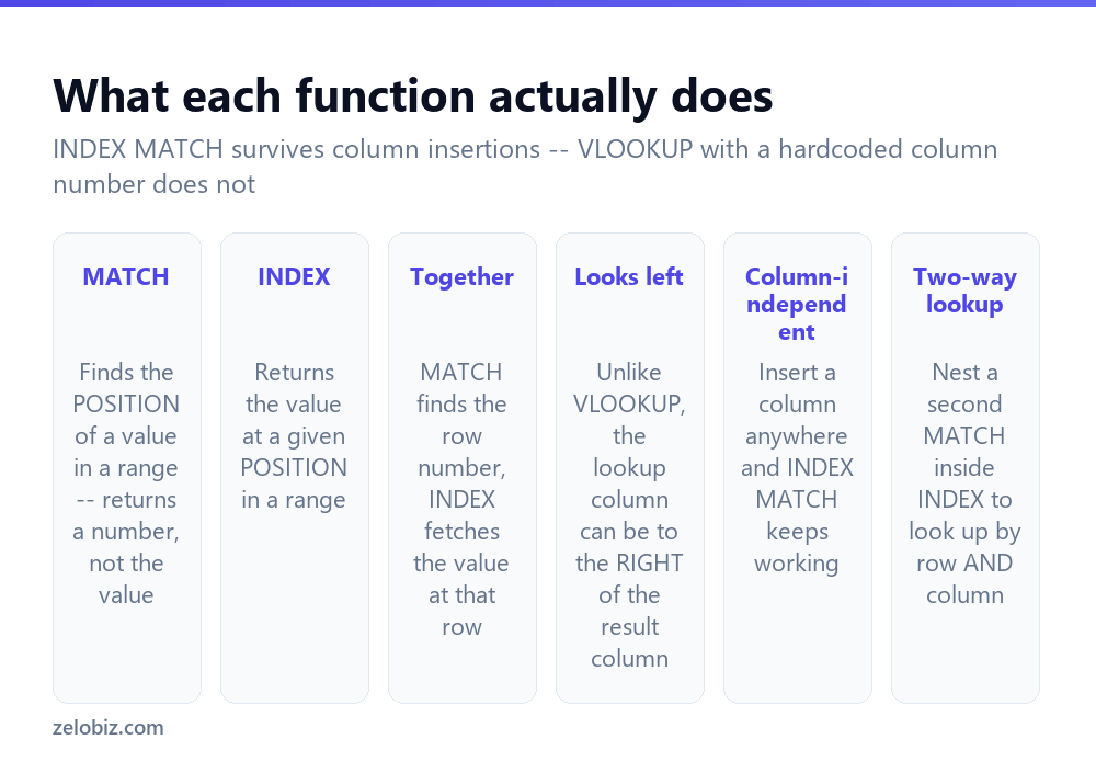
They’re two unrelated functions that happen to combine well, so it helps to understand each one alone before nesting them.

MATCH(lookup_value, lookup_array, match_type) searches a range and returns a position number, not the value itself. =MATCH("Widget",A1:A10,0) might return 4, meaning “Widget” is the 4th item in that range — it tells you nothing about what’s in any other column.

INDEX(array, row_num) returns the value at a given position in a range. =INDEX(C1:C10,4) returns whatever is in the 4th row of column C. On its own it needs a row number you already know.

Combining them

Nest the MATCH formula inside INDEX, in place of the row number: =INDEX(C:C, MATCH("Widget",A:A,0)).

Read it right to left: MATCH finds which row “Widget” occupies in column A, then INDEX returns column C’s value from that same row. The 0 at the end of MATCH means exact match — almost always what you want, and easy to forget.

Replace the hardcoded “Widget” with a cell reference to make it reusable: =INDEX(C:C,MATCH(F1,A:A,0)) looks up whatever value is typed into F1, updating automatically as F1 changes.

Building it step by step

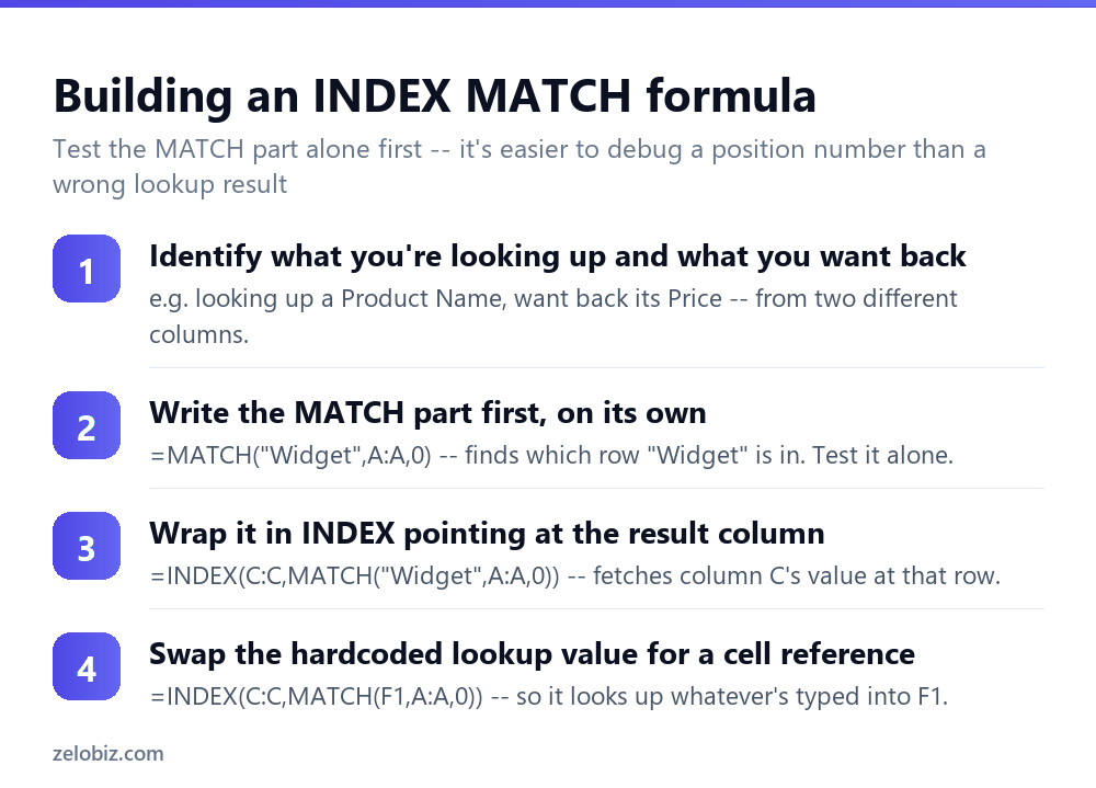
Write and test the MATCH part in an empty cell by itself first: =MATCH("Widget",A:A,0). If it returns a sensible row number, the lookup logic is correct. If it returns #N/A, fix that before adding INDEX — debugging a bare number is much easier than debugging a wrong lookup result.

Once MATCH works, wrap it inside INDEX pointing at the column you actually want returned. Then swap the hardcoded lookup value for a cell reference so the formula becomes reusable rather than a one-off.

Why INDEX MATCH over VLOOKUP

VLOOKUP works fine for simple cases, but INDEX MATCH solves three of its real limitations:

The biggest practical difference is the middle row of that table. VLOOKUP’s third argument is a column number — 3 means “the third column in the range”. Insert a new column anywhere inside that range and every VLOOKUP using a hardcoded number now points at the wrong column, with no error to flag it. INDEX MATCH references the result column directly, so it keeps pointing at the right data regardless of what gets inserted around it.

Two-way lookup: row and column

Nesting a second MATCH inside INDEX looks up a value by both a row criteria and a column criteria at once — useful for a grid like months across the top and products down the side.

=INDEX(B2:M20, MATCH("Widget",A2:A20,0), MATCH("March",B1:M1,0)). The first MATCH finds which row “Widget” is in; the second finds which column “March” is in; INDEX returns the value at that row-and-column intersection. This is something VLOOKUP cannot do at all without a helper column.

A worked example

Say column A holds Product Name, column B holds Category, and column C holds Price, across 150 rows. A cell F1 has a product name typed into it, and F2 should show its price.

=INDEX(C:C,MATCH(F1,A:A,0)). MATCH searches column A for whatever’s in F1 and returns its row position — say, 47. INDEX then returns the 47th value in column C. Change F1 to a different product name and the whole thing recalculates instantly.

Now suppose the layout changes and Category needs to sit between Product Name and Price — a new column is inserted at B, pushing Price to column D. A VLOOKUP using a hardcoded column number 3 would now return the wrong column silently. The INDEX MATCH formula above needs no change at all, because it references column C by its actual column reference at the time of the insert — Excel automatically updates C:C to D:D when a column is inserted before it, the same way it would update any other formula’s cell references.

Approximate match: the other use for MATCH

The third MATCH argument isn’t always 0. Setting it to 1 finds the largest value less than or equal to the lookup value, provided the range is sorted ascending — useful for tax brackets, shipping-rate tiers, or grade boundaries where you want “the bracket this number falls into” rather than an exact match.

Setting it to -1 does the reverse — finds the smallest value greater than or equal to the lookup value, in a descending-sorted range. Both of these are considerably less common than exact match (0), and both require the data to actually be sorted correctly or the result is unreliable, which is why exact match is the safer default unless you specifically need a bracket lookup.

Using named ranges to make it more readable

A formula like =INDEX(C:C,MATCH(F1,A:A,0)) is fine on the sheet it was written on, but column letters alone don’t say what the data actually is. Defining named ranges — select column A, type Prices_Lookup into the Name Box, Enter — lets the same formula read as =INDEX(Prices_Values,MATCH(F1,Prices_Lookup,0)), which is self-documenting to anyone opening the sheet later, including a future version of yourself. This matters more as a workbook grows past a handful of formulas that all look alike.

Common errors and what they mean

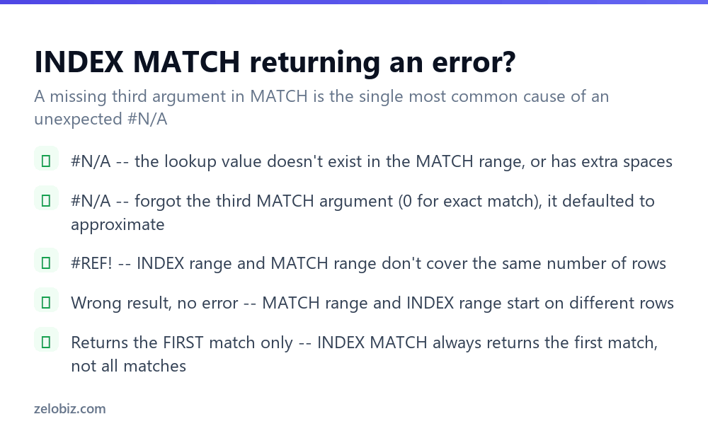
#N/A from MATCH means the lookup value genuinely isn’t found in the range — check for trailing spaces or a mismatch between text and number formatting (a product code stored as text in one column and as a number in the other won’t match).

#N/A that seems wrong — you’re confident the value exists — almost always means the third MATCH argument was left out. Without it, MATCH defaults to approximate match, which requires the range to be sorted and often returns #N/A on unsorted data instead of the exact match you expected. Always include the 0.

#REF! error means the INDEX range and the MATCH range don’t line up in size — MATCH returned a position that falls outside the INDEX range. Check both cover the same rows.

A result with no error, but clearly wrong — usually the INDEX range and MATCH range start on different rows. If MATCH searches A2:A100 but INDEX returns from C1:C99, every result is off by one row.

Frequently asked questions