

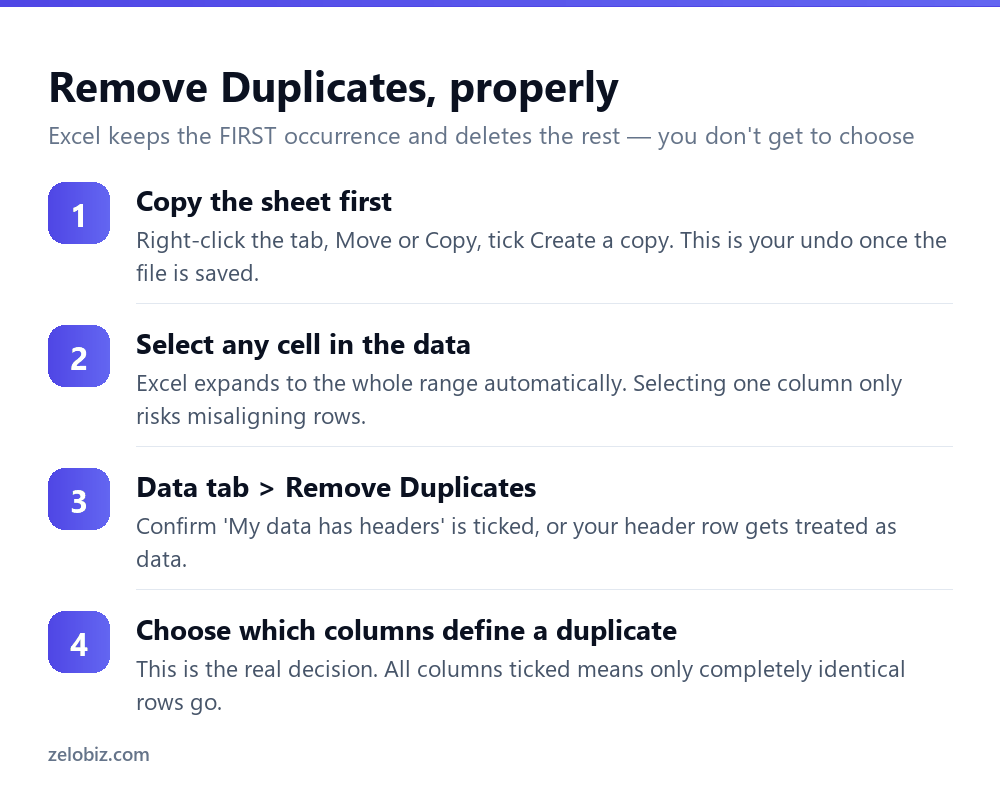
To remove duplicates in Excel, click any cell in your data, go to the Data tab and click Remove Duplicates. Tick the columns that define a duplicate and click OK. Two things to know first: Excel deletes the rows immediately and keeps the first occurrence of each, and once you save and close the file there’s no undo. Copy the sheet before you start.
What Excel does that nobody mentions
Remove Duplicates is a single button and it works. It’s also more destructive than its friendly dialog suggests, in three specific ways.
It keeps the first occurrence. If row 4 and row 40 are duplicates, row 4 survives and row 40 is deleted. You don’t get to choose, and if row 40 held the more recent or more complete version, it’s gone. Sort your data before removing so the row you want to keep is the one nearer the top.
It tells you a count, not what it deleted. You get ’17 duplicate values found and removed’ with no list of what those were. If the count surprises you, there’s no way to look at what went.
Undo expires. Ctrl+Z works within the session. Save and close, and the deleted rows are unrecoverable.
Copy the sheet before you click Remove Duplicates. It takes four seconds and it’s the only real safety net Excel gives you.
Choosing which columns define a duplicate
This is the part people skim, and it changes the result completely.
Excel ticks every column by default, meaning a row is only a duplicate if every single field matches. In a customer list where the same person appears twice with slightly different phone numbers, nothing is removed — the rows aren’t identical.
Usually you want to define duplicates by a smaller set. Tick Email alone and any repeated email address is treated as a duplicate regardless of what else differs. Tick First name and Last name together and you catch the same person entered twice.
⚠️ Watch out: Never select a single column of a wider table and remove duplicates from it. Excel offers to continue with just that column, and if you accept, it deletes cells from that column only and shifts them up — misaligning every row against its neighbours. Always click a single cell and let Excel expand the selection.
Look before you delete
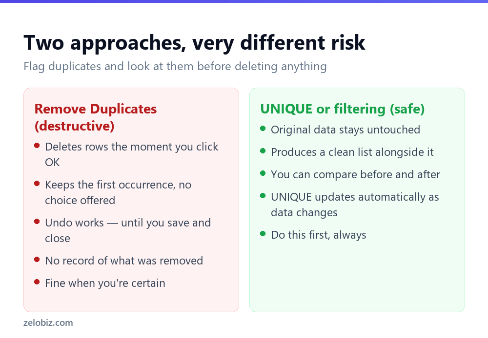
The safer sequence is to find duplicates first, look at them, then decide. Two ways, both non-destructive.
Highlight them with conditional formatting
Select your column, then Home › Conditional Formatting › Highlight Cells Rules › Duplicate Values. Every repeated value turns red. Nothing is changed — you can now scroll through and see exactly what Excel would remove, and whether that’s what you want.
Worth knowing this highlights all occurrences including the first, so three copies of a value show three red cells rather than two.
Count them with COUNTIF
In a spare column, =COUNTIF(A:A,A2) returns how many times the value in A2 appears in the whole column. Anything above 1 is duplicated. Filter that column to greater than 1 and you have a working list of every duplicate, with its row still attached.
This is the version to use when you need to investigate rather than just clean — it tells you how many times something repeats, not just that it does.
UNIQUE: the non-destructive answer
In Microsoft 365 and Excel 2021 onwards, =UNIQUE(A2:A100) returns a deduplicated list in a new location. Your original data isn’t touched at all.
Because it’s a formula, it also stays current. Add rows to the source and the unique list updates itself. That makes it the right choice for a working spreadsheet rather than a one-off clean.
It works across multiple columns too: =UNIQUE(A2:C100) returns unique rows across all three columns. And a useful variant — =UNIQUE(A2:A100,,TRUE) — returns only values that appear exactly once, discarding anything repeated, which is occasionally exactly what you need.
💡 Pro tip: Older Excel without UNIQUE? Copy the column to a blank sheet, run Remove Duplicates there, and you’ve got the same result with the original untouched.
When Excel misses obvious duplicates
The most common complaint: two cells look identical, Excel disagrees. It’s almost always invisible characters.
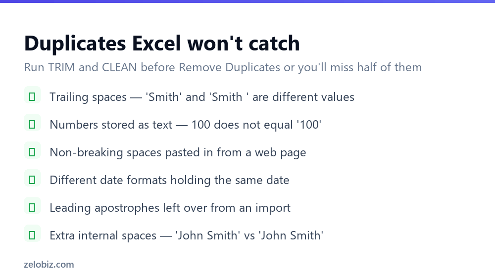
Trailing spaces are the usual culprit, especially in data exported from another system. ‘Smith’ and ‘Smith ‘ are genuinely different values as far as Excel is concerned. Fix the whole column with =TRIM(A2), which strips leading and trailing spaces and collapses internal doubles to single.
Numbers stored as text is the second. A cell containing the text ‘100’ will never match a cell containing the number 100, and the only visual clue is the alignment — text sits left, numbers right. Look for the small green triangle in the corner, or check whether the column aligns inconsistently.
Data pasted from a web page often carries non-breaking spaces, which TRIM won’t remove because they’re technically a different character. =TRIM(CLEAN(SUBSTITUTE(A2,CHAR(160)," "))) handles all three problems at once and is worth keeping to hand.
Case sensitivity
Remove Duplicates is case-insensitive. ‘SMITH’, ‘Smith’ and ‘smith’ are treated as the same value, and Excel keeps whichever appeared first.
That’s usually helpful and occasionally wrong — product codes and passwords are cases where AB123 and ab123 may be genuinely different records. There’s no setting to change this.
If case matters, add a helper column with =EXACT(A2,A3) after sorting, or use =SUMPRODUCT(--EXACT(A:A,A2)) to count case-sensitive matches. Then deduplicate on that helper column instead.
Duplicates across two sheets
Remove Duplicates only works within one range. To find records in Sheet1 that also appear in Sheet2, use a lookup.
=COUNTIF(Sheet2!A:A,A2) returns how many times the value in Sheet1’s A2 appears anywhere in Sheet2’s column A. Zero means it’s unique to Sheet1; anything higher means it exists in both. Filter on that and you can remove, keep or investigate as you choose.
For matching on several fields at once, concatenate them into a key first — =A2&"|"&B2&"|"&C2 in both sheets — and COUNTIF against that. The pipe separator prevents false matches where fields run together.
Power Query, for anything you’ll repeat
If you deduplicate the same export every week, doing it by hand every time is the wrong tool. Power Query records the steps once and replays them.
Select your data, go to Data › From Table/Range, then right-click the column heading and choose Remove Duplicates. Click Close & Load and you get a clean table on a new sheet. Next month, paste the new export over the source and hit Refresh — the same cleaning runs automatically.
It also does things the plain button can’t: trim whitespace, change case, and remove duplicates all as recorded steps, in order. And it never touches your source data, so there’s nothing to undo.
Duplicates in a Pivot Table
A different problem worth separating: sometimes you don’t want to delete duplicates, you want to count distinct values.
In a Pivot Table, right-click any value field, choose Value Field Settings, and pick Distinct Count. That tells you how many unique customers placed orders rather than how many orders there were — usually the number people actually want.
Distinct Count only appears if you tick Add this data to the Data Model when creating the Pivot Table. If the option is missing, that’s why, and you’ll need to recreate the pivot with that box ticked.
- ✓Copy the sheet before removing anything
- ✓Sort so the row you want to keep is nearest the top
- ✓Highlight duplicates and look at them first
- ✓Run TRIM and CLEAN before deduplicating imported data
- ✓Use UNIQUE for anything you’ll update again later
- ✕Selecting one column of a wider table and removing duplicates
- ✕Leaving all columns ticked when you mean ‘same email’
- ✕Assuming undo will save you after saving and closing
- ✕Expecting Excel to distinguish uppercase from lowercase
- ✕Deleting before checking why the count is higher than expected
Frequently asked questions
How do I remove duplicates in Excel?
Click any cell in your data, go to the Data tab and click Remove Duplicates. Tick the columns that define a duplicate, then click OK. Excel keeps the first occurrence of each and deletes the rest immediately.
Does Remove Duplicates keep the first or last row?
The first. Excel scans top to bottom and keeps the first occurrence it finds. If you need to keep the most recent entry instead, sort your data so that one appears highest before running it.
Why is Excel not finding my duplicates?
Usually invisible characters — trailing spaces, non-breaking spaces from a web paste, or numbers stored as text. Clean the column first with =TRIM(CLEAN(SUBSTITUTE(A2,CHAR(160),” “))) and try again.
How do I find duplicates without deleting them?
Use Home, Conditional Formatting, Highlight Cells Rules, Duplicate Values to colour them, or add a column with =COUNTIF(A:A,A2) and filter for values above 1.
Is Remove Duplicates case sensitive?
No. Excel treats SMITH, Smith and smith as identical. If case matters, build a helper column using EXACT and deduplicate on that instead.
Can I undo Remove Duplicates?
Only within the same session, with Ctrl+Z. Once the file is saved and closed the deleted rows cannot be recovered. Copy the sheet before you start.
- →Tidy the layout without breaking things — how to merge cells in Excel
- →Protect the formulas: how to lock cells in Excel
- →Bring back missing data with how to unhide columns in Excel
- →Match records across sheets: how to use VLOOKUP