

To use SUMIF in Excel, type =SUMIF(range, criteria, sum_range) — range is the column checked against your condition, criteria is what to match, and sum_range is the column of numbers to add up. For example, =SUMIF(B:B,"Food",D:D) adds every value in column D where column B says “Food”. For more than one condition, use SUMIFS instead.
The Gap Every Guide Leaves Out: How to Use a Cell as Your SUMIF Threshold
Nearly every SUMIF example, including Microsoft’s own reference page, types the comparison value straight into the formula: ">100". That’s fine for a one-off check you’ll run once and forget about. It falls apart the moment the number needs to change monthly, because updating a hardcoded threshold means opening and editing the formula itself, and formulas that get hand-edited often are formulas that eventually get typo’d.
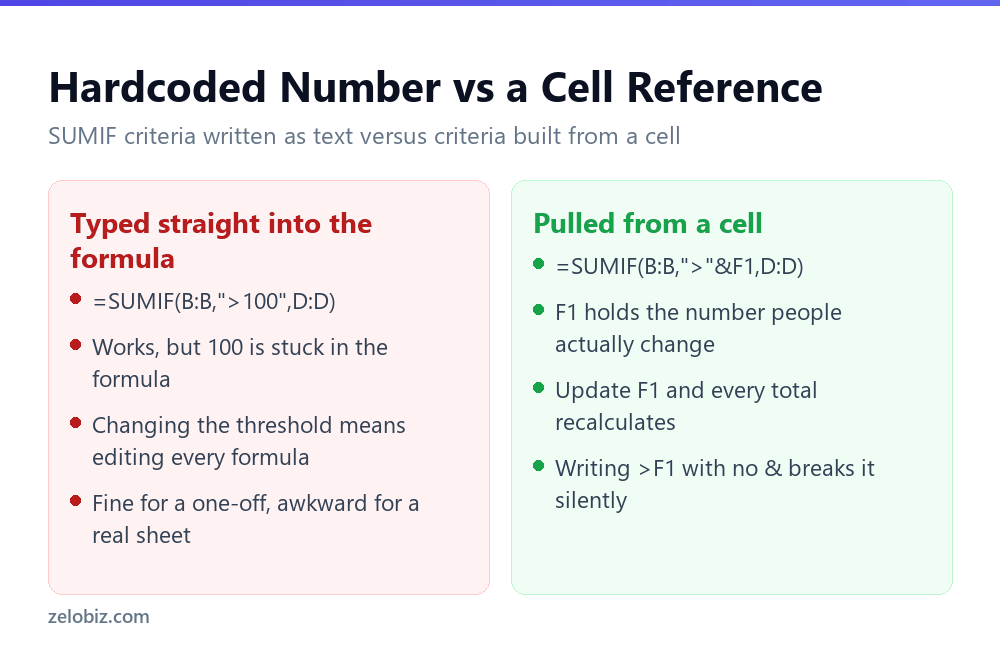
Once that pattern clicks, it works anywhere a static operator would: =SUMIF(B:B,"<"&F1,D:D) for below a moving threshold, or with a date cell instead of a number, =SUMIF(C:C,">"&F2,D:D) where F2 holds a cutoff date someone can change without touching the formula bar at all. Put the threshold in a labelled cell above your data, point every SUMIF at that cell through the ampersand, and the whole sheet of totals updates itself the moment that one number changes, with nothing else to touch.
⚠️ Watch out: Only the operator goes inside the quotes. ">"&F1 is correct. ">F1" puts the cell reference inside the quotes and breaks it, and &">F1" with the ampersand in the wrong place does too. It’s a small formatting detail that’s easy to get backwards under time pressure, and it’s probably the single most common reason someone reports that a working SUMIF formula “stopped working” right after they tried to make it more flexible and dynamic.
The three arguments, in the order that matters
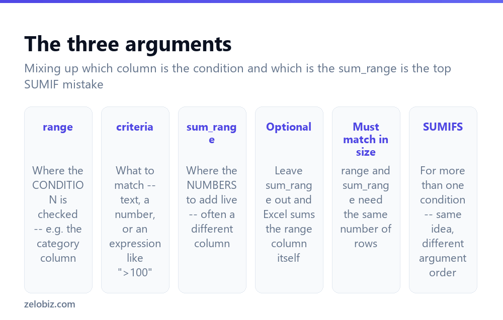
=SUMIF(range, criteria, [sum_range]). The part people get backwards is that range is where the condition lives, and sum_range is where the numbers to total live — they’re frequently two different columns entirely.
If you want the total of column D wherever column B says “Food”: B is your range (that’s what gets checked), “Food” is your criteria, and D is your sum_range (that’s what gets added). Written out: =SUMIF(B:B,"Food",D:D).
sum_range is optional. Leave it out and SUMIF sums the range column itself — useful when the condition and the numbers are in the same column.
Text, number, and expression criteria
Criteria can be an exact value, a comparison, or a wildcard pattern, and each is written slightly differently:
=SUMIF(B:B,"Food",D:D)— exact text match=SUMIF(B:B,">100",D:D)— numbers greater than 100 (operator inside quotes)=SUMIF(B:B,"*shirt*",D:D)— text containing “shirt” anywhere=SUMIF(B:B,A1,D:D)— match whatever value is in cell A1=SUMIF(F:F,">="&DATE(2026,3,1),D:D)— dates on or after March 1, 2026
The pattern with an operator is the one people write wrong most often: the operator has to be inside the quotes, as part of the text string — ">100", never >100 on its own.
Writing the formula step by step
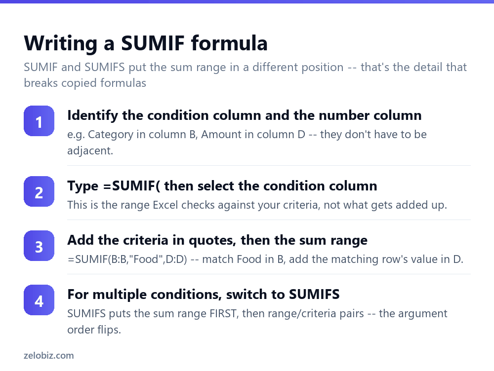
Slow down for the first one you write in a new sheet, because the argument order is easy to get backwards under time pressure.
Identify which column holds what you’re filtering by, and which holds the numbers you actually want totalled. They can be next to each other or far apart — SUMIF doesn’t care about their relative position, only that both ranges cover the same rows.
Then build the formula left to right exactly as the function expects it: range, criteria, sum_range. Reading it back as a sentence helps — “sum column D, where column B equals Food.”
SUMIFS: more than one condition
SUMIF only takes a single condition. For “total sales where Category is Food AND Region is West”, use SUMIFS — and note the argument order flips.
=SUMIFS(sum_range, range1, criteria1, range2, criteria2, ...). The sum range comes first in SUMIFS, not last like in SUMIF. That’s the detail that breaks a formula copied from one function to the other without adjusting the order.
Example: =SUMIFS(D:D,B:B,"Food",C:C,"West") — sum column D, where B is Food AND C is West. Every condition must be true for a row to be included; there’s no built-in OR.
A worked example
Say column B holds a category (“Food”, “Drink”, “Household”) for 300 expense rows, column C holds the date, and column D holds the amount. A few real questions and the formula for each:
Total spent on Food: =SUMIF(B2:B301,"Food",D2:D301). One condition, one sum column.
Total spent on Food in March: two conditions now, so SUMIF alone can’t do it — =SUMIFS(D2:D301,B2:B301,"Food",C2:C301,">="&DATE(2026,3,1),C2:C301,"<"&DATE(2026,4,1)). Three range/criteria pairs: category, start date, and end date, all of which must be true together.
Total spent on anything except Household: there's no "not equal" shortcut built into a single SUMIF for excluding one category among several, so the practical route is to sum everything and subtract the excluded category: =SUM(D2:D301)-SUMIF(B2:B301,"Household",D2:D301).
Average spend per Food transaction: SUMIF only totals, it doesn't average matching rows on its own. Combine it with COUNTIF: =SUMIF(B2:B301,"Food",D2:D301)/COUNTIF(B2:B301,"Food"). Excel also has a dedicated AVERAGEIF function that does the same thing in one call.
Working through questions like these one at a time, checking each total against a manual filter-and-glance of the data, is the fastest way to catch a misaligned range before it feeds into something larger.
SUMIF with an OR condition across values
SUMIFS requires every condition to match -- there's no built-in way to say "Food OR Drink" inside a single set of SUMIFS arguments. The common workaround is an array constant: =SUM(SUMIF(B:B,{"Food","Drink"},D:D)). The curly braces hold a list of values, SUMIF evaluates the sum for each one individually, and the outer SUM adds those results together. It reads oddly the first time but scales better than writing out SUMIF(...)+SUMIF(...) by hand for a longer list of values.
Why SUMIF returns 0
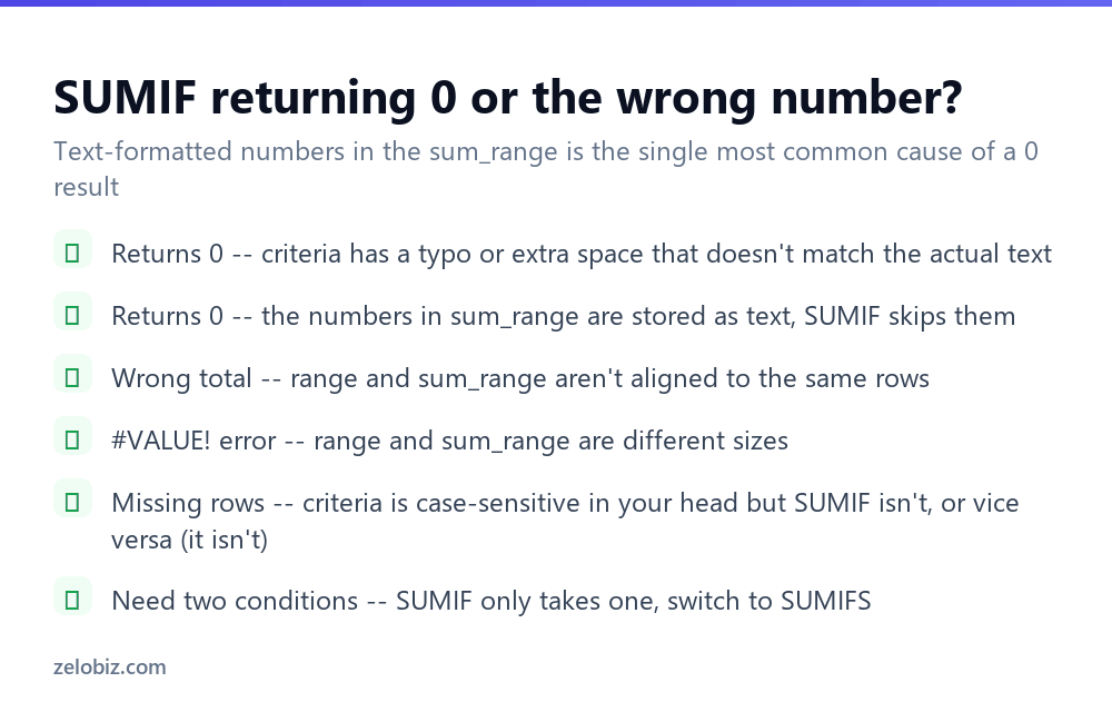
Numbers stored as text is the most common cause. SUMIF, like SUM, ignores text-formatted numbers entirely in the sum_range -- they show as left-aligned with a green triangle in the corner. Convert them with Data › Text to Columns › Finish, which forces a re-evaluation of the cell type without changing the values.
A criteria typo or trailing space is the second most common cause. "Food " with a trailing space won't match "Food" as a criteria string, even though it looks identical in the cell. Copy the exact text from the source column rather than retyping it if a match is failing unexpectedly.
Misaligned ranges -- if range is B2:B100 but sum_range is D1:D99, SUMIF checks B2 but sums D1, one row off from where you intended. Both ranges need to start and end on the same rows.
SUMIF is not case-sensitive
Text criteria in SUMIF ignore letter case entirely -- "food", "Food", and "FOOD" all match the same rows. This is rarely a problem in practice, but it does mean SUMIF can't be used to distinguish two categories that differ only in capitalisation, which occasionally comes up in data imported from a system that used case to mean something (a product code entered in lowercase versus uppercase to flag a different batch, for example). If that distinction matters, a helper column using the case-sensitive EXACT function is the workaround, since SUMIF itself has no case-sensitive mode.
SUMIF with dates
Date criteria are a common stumbling block because typing a date directly into the criteria string doesn't reliably work across regional date formats.
The reliable pattern uses DATE() and string concatenation: =SUMIF(F:F,">="&DATE(2026,3,1),D:D) sums D wherever the date in F is on or after March 1, 2026. For a range between two dates, combine two SUMIFS conditions rather than one SUMIF, since you need both a lower and upper bound.
💡 Pro tip: For anything with a date range, reach for SUMIFS even if there's technically only one column being filtered -- 'on or after X' and 'before Y' are two separate conditions.
The same operator-plus-cell pattern from earlier works here too. Swap the fixed DATE() for a cell holding a cutoff date, or for TODAY() when the cutoff is "now" rather than a fixed day: =SUMIF(F:F,">="&TODAY()-30,D:D) sums anything from the last 30 days and keeps working tomorrow without anyone touching the formula, since TODAY() moves forward on its own.
SUMIF referencing a Table instead of a full column
Using an entire column reference like B:B works fine, but it means Excel checks every one of a million-plus rows on every recalculation, even the empty ones below your actual data. On a small sheet that's invisible; on a large one with many formulas it adds up.
Converting the source range to an Excel Table (Ctrl+T) and writing the formula against the Table's structured references solves both problems at once: =SUMIF(Table1[Category],"Food",Table1[Amount]) only evaluates actual data rows, and it expands automatically as new rows are added -- no editing the formula's range later. This is the version worth using for anything that will keep growing, like a running expense log or an order list that's added to daily.
SUMIF vs SUMPRODUCT vs a PivotTable
SUMIF is the right tool for a single running total that updates live in a cell. Three situations call for something else:
Complex logic -- an OR condition, or a calculation combining several columns -- is easier in SUMPRODUCT, which can evaluate arbitrary boolean expressions across multiple arrays.
Several different breakdowns at once -- total by category, by region, and by month, all from the same data -- is what a PivotTable is for. Writing nine separate SUMIFS formulas to replicate a three-by-three breakdown works but doesn't scale.
A running dashboard number that just needs to update automatically as new rows are added is exactly SUMIF's job, especially if the range references a Table so it expands automatically.
- ✓Remember range=condition, sum_range=numbers to add
- ✓Put operators inside the quotes: ">100"
- ✓Switch to SUMIFS the moment you need a second condition
- ✓Convert text-formatted numbers before summing them
- ✓Reference an Excel Table so the range grows automatically
- ✕Assuming SUMIF and SUMIFS take arguments in the same order
- ✕Typing >100 without quotes
- ✕Letting range and sum_range cover a different number of rows
- ✕Typing a date directly into criteria instead of using DATE()
- ✕Writing nine SUMIFS formulas when a PivotTable would replace all of them
Worked example: a budget alert that updates itself
A small team wants a single cell showing total spend on any expense line over budget, where "over budget" is a number that gets revised every quarter.
Cell F1 holds the budget figure, say 500, labelled clearly so anyone opening the sheet knows what it controls. The formula in F2 is =SUMIF(C:C,">"&F1,C:C), which totals every amount greater than whatever sits in F1. With the sample data above that returns 1,620, the sum of Software and Equipment, since both exceed 500 and Travel doesn't.
Change F1 to 700 next quarter and F2 recalculates to 980 on its own, no formula editing involved. That's the entire point of routing the threshold through a cell: the person updating the budget number doesn't need to know SUMIF exists, let alone how to edit one correctly, and nobody has to remember to touch the formula again.
This scales past one condition too. Add a second criteria pair to turn it into SUMIFS, and the same F1 cell can gate a multi-condition total just as easily as a single one, matching everything covered under SUMIFS above.
It's worth being deliberate about where that threshold cell lives. Burying it in the middle of a data table invites someone to overwrite it by accident while sorting or filtering. Putting it in a clearly labelled cell near the top of the sheet, with a short note like "Budget threshold" next to it, means the next person to open the file understands what controls the total without having to click into F2 and reverse-engineer the formula.
The same goes for any workbook you didn't build yourself. Before assuming a SUMIF is hardcoded, click the cell and check whether the number in the formula bar is a literal value or a reference dressed up with an ampersand. It's a five-second check that saves the embarrassment of editing a formula that was already built to be flexible.
Frequently asked questions
How do I make SUMIF compare against a cell instead of a fixed number?
Join the operator and the cell with an ampersand, keeping only the operator inside quotes: =SUMIF(range,">"&F1,sum_range). Writing ">F1" instead puts the cell reference inside the quotes, so Excel treats it as literal text and the formula returns 0.
What is the syntax for SUMIF in Excel?
=SUMIF(range, criteria, sum_range). range is the column checked against criteria, and sum_range is the column of numbers to add up for matching rows.
Why does SUMIF return 0?
Usually because the numbers in sum_range are stored as text, or the criteria has a typo or trailing space that doesn't exactly match the source data.
What's the difference between SUMIF and SUMIFS?
SUMIF takes one condition and puts sum_range last. SUMIFS takes multiple conditions (all must match) and puts sum_range first.
How do I use SUMIF with a date range?
Use SUMIFS with two conditions: >= the start date and < the end date, each written as ">="&DATE(year,month,day) to avoid regional date format issues.
Can SUMIF use an OR condition?
Not directly. Add two separate SUMIF formulas together, one per condition, e.g. =SUMIF(B:B,"Food",D:D)+SUMIF(B:B,"Drink",D:D).
Does SUMIF work with wildcards?
Yes. Use * to match any text, e.g. "*shirt*" matches any cell containing the word "shirt" anywhere in it.
- →Count instead of sum: how to count cells in Excel
- →Multiple breakdowns at once: how to make a pivot table in Excel
- →Look up a value by two criteria: how to use INDEX MATCH in Excel
- →Highlight the totals automatically: how to use conditional formatting in Excel