How to Unhide Rows in Excel (Row 1 Never Works the Normal Way)

The normal way to unhide rows in Excel stops working the moment row 1 is the one that’s hidden. So the usual right-click trick just doesn’t show the option.

That’s not a bug. It’s a direct result of how the selection method works. Once you see why, the fix takes seconds.

The Normal Method

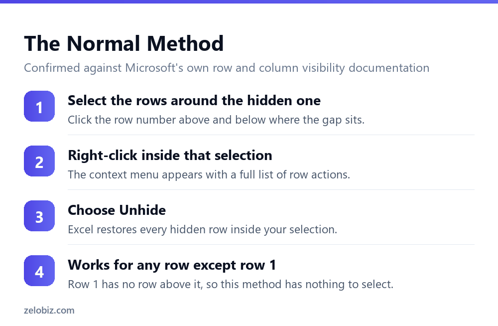
For most hidden rows, unhiding is simple. Click the row number just above the gap. Hold Shift and click the row number just below it. That selects both visible neighbors, with the hidden row trapped in between.

Right-click anywhere inside that selection. Excel shows a full context menu, including Unhide. Click it, and every hidden row inside your selection reappears.

Why Row 1 Is Different

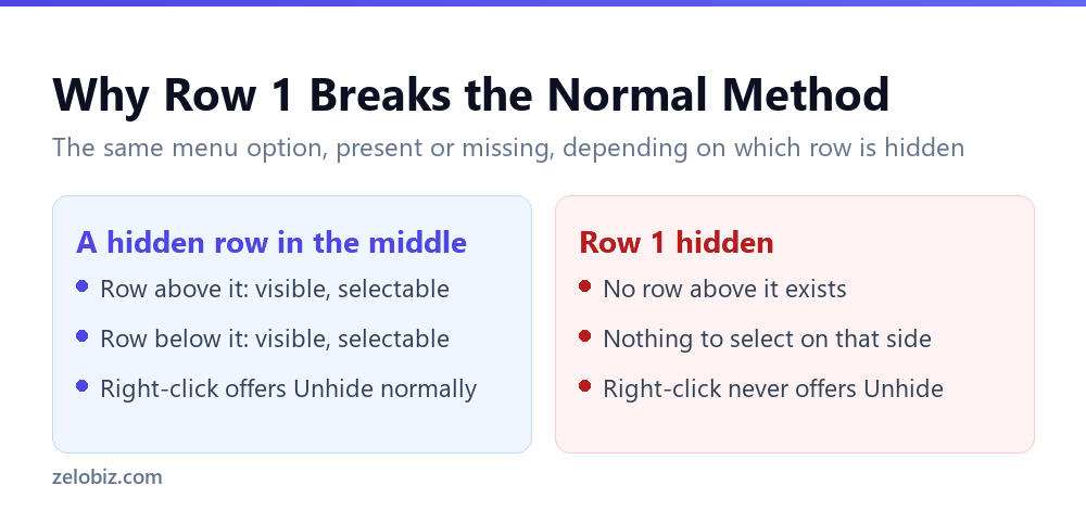
So the entire normal method depends on selecting a visible row on each side of the hidden one. For a hidden row in the middle of a sheet, that’s trivial.

But row 1 sits at the very top. There’s no row 0. So there’s nothing to click on that side, and the selection Excel needs to offer Unhide simply can’t be made the normal way.

The Fix for Row 1

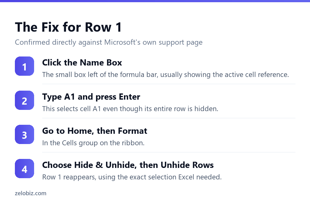
Because row 1 can’t be selected by clicking, Excel needs a different way to select it. The Name Box provides exactly that.

Click the Name Box, the small field just left of the formula bar. Type A1 and press Enter. Excel selects cell A1 directly by name, even though the entire row is hidden and invisible.

With that selection active, go to the Home tab. In the Cells group, click Format. Choose Hide & Unhide, then Unhide Rows. Row 1 reappears immediately.

An equivalent path works too: Home, Find & Select, Go To. Type A1 in the Reference box, click OK. That selects the same cell, and the same Format menu steps finish the job.

Unhiding Everything at Once

So what if several rows are hidden across a sheet, and tracking down each one individually feels tedious? A faster method exists.

Click the small triangle in the corner where the row numbers and column letters meet, just above row 1 and left of column A. That selects the entire worksheet at once, hidden rows included.

With everything selected, use the keyboard shortcut. On Windows desktop Excel, that’s Ctrl+Shift+( , the left parenthesis, produced by holding Shift and pressing 9 on a standard keyboard. Excel for the web documents this same action simply as Ctrl+Shift+9.

What Actually Hides a Row

So it helps to know how a row gets hidden in the first place, since it affects how you find it again. Someone can hide a row deliberately, through the same Format menu, or by dragging a row’s height down to zero.

Both produce the same visual result: the row disappears, and the row numbers skip straight from one number to the next. But there’s no visual marker in the row headers themselves showing exactly which rows are missing, only the number gap.

That gap is the tell. If row numbers jump from 4 to 6, row 5 is hidden somewhere in between, whether it was hidden through the menu or by a dragged row height.

Troubleshooting When the Fix Doesn’t Work

So occasionally, the Name Box method doesn’t immediately fix things. A few specific causes explain most of those cases.

First, check whether row heights were set to zero instead of hidden through the menu. Both look identical on screen, but a zero-height row sometimes needs its height reset directly, through Format, Row Height, rather than Unhide.

Second, confirm the worksheet itself isn’t protected. A protected sheet can block row and column changes entirely, including unhiding, until protection is removed from the Review tab.

Third, double-check you actually typed A1 into the Name Box and pressed Enter, not just clicked near it. The selection has to register before the Format menu options will act on the right row.

A Worked Example, Start to Finish

So picture opening a shared budget spreadsheet and noticing the row numbers jump straight from 1 to 4. Rows 2 and 3 are hidden.

Because row 1 is visible here, not hidden, the normal method works fine. Select rows 1 and 4 together, right-click, choose Unhide, and rows 2 and 3 both reappear at once.

Now imagine the same sheet, but row 1 itself is the one hidden, so the numbers start at 2. That’s exactly the case the normal method can’t handle, and where the Name Box fix becomes necessary instead.

Telling the two situations apart takes one glance at the row numbers. If they start at 1, the normal method will work for whatever’s hidden further down. If they start above 1, row 1 itself is hidden, and the Name Box method is what’s needed.

Why This Trips Up Row 1 Specifically

So it’s worth asking why this particular edge case exists at all, instead of Excel just handling it automatically.

Excel’s right-click Unhide relies entirely on a selection spanning the hidden rows. That’s a consistent, simple rule that works correctly for every row except the very first one, where the rule runs out of rows to include.

Rather than special-casing row 1 inside the right-click menu, Excel expects users to reach it through direct cell selection instead, which the Name Box and Go To both provide. It’s a design tradeoff, not an oversight.

Unhiding a Specific Block of Rows, Not Everything

So sometimes the goal isn’t unhiding every row on the sheet, just a specific block buried somewhere in the middle. The select-all shortcut works, but it also reveals rows that were deliberately hidden for a different reason.

For a targeted fix, select a wider range that safely includes the hidden block, rows 8 through 15 for example, even if the hidden rows only span 10 through 12. Right-click inside that selection and choose Unhide.

Excel unhides every hidden row inside the selected range, but leaves rows outside that range untouched. So a wide-but-bounded selection is the safer middle ground between fixing one row at a time and unhiding the entire sheet at once.

How This Compares to Filtering

So it’s worth being clear about a related but different feature: filtering. A filtered-out row and a hidden row look identical, both simply missing from view, but they behave very differently.

A filter temporarily hides rows based on a condition, and clearing the filter brings every row back instantly, no Format menu required. A manually hidden row stays hidden regardless of any filter, until it’s specifically unhidden.

If unhiding through the methods in this article doesn’t work, checking whether a filter is active, visible as a funnel icon on the column headers, rules out a second, unrelated cause of the same symptom.

Common Questions

The Short Version

Hiding a Row on Purpose

So it’s worth covering the other direction too, since knowing how a row gets hidden makes it easier to recognize later. Select the row or rows you want to hide, right-click the row number, and choose Hide.

That’s the entire process. No confirmation dialog, no warning. The row simply disappears, and the row numbers jump straight past it, which is the same visual signature covered earlier in this article.

Because hiding takes one click and leaves no obvious trace beyond the number gap, it’s easy for someone to hide a row temporarily, forget about it, and leave a shared sheet with a row missing that nobody remembers hiding on purpose.

A Faster Habit for Frequent Use

So for anyone who hides and unhides rows often, memorizing two shortcuts replaces most of the menu navigation entirely.

Select the rows to hide, then press Ctrl+9. To unhide a selection that spans the hidden rows, press Ctrl+Shift+( instead. Both skip the right-click menu and the Format ribbon path completely.

For row 1 specifically, the Name Box selection still comes first, since there’s no way to select a hidden row 1 by clicking. But once A1 is selected through the Name Box, Ctrl+Shift+( finishes the job just as fast as the Format menu does.

If the Whole Sheet Feels Wrong, Not Just One Row

So occasionally, what looks like a hidden-row problem is actually something else entirely: frozen panes, split windows, or a very large row height set to nearly zero rather than fully hidden.

Frozen panes can make it look like rows are missing near a scroll boundary, when they’re really just locked in place above where you’re scrolled to. Checking the View tab for an active freeze setting rules that out quickly.

A row height set to something like 1 or 2 pixels, rather than fully hidden through the Format menu, looks nearly identical to a hidden row but responds differently. Right-click and Unhide won’t restore it, since technically it was never hidden. Format, Row Height, and typing in a normal value like 15 fixes that case instead.

So between hidden rows, frozen panes, and near-zero row heights, three different causes can produce a similar-looking gap. Checking each in turn, rather than guessing, gets to the right fix faster than trial and error.