The VLOOKUP Mistake That Breaks a Column With No Error

A VLOOKUP formula that worked yesterday can go quietly wrong today. No error, no red flag. Just the wrong number sitting in a cell that looks completely normal.

The usual cause is one specific action: someone inserted a column somewhere inside the lookup range. Here’s exactly why that breaks VLOOKUP, how it differs from other failures, and what actually fixes it.

What VLOOKUP’s Four Arguments Actually Do

VLOOKUP takes four arguments. The syntax is VLOOKUP(lookup_value, table_array, col_index_num, [range_lookup]).

That third argument is the one that causes trouble. It’s just a number. VLOOKUP has no idea what column header that number is supposed to represent. It only knows “count this many columns over from the left edge of my range.”

Why an Inserted Column Breaks It Silently

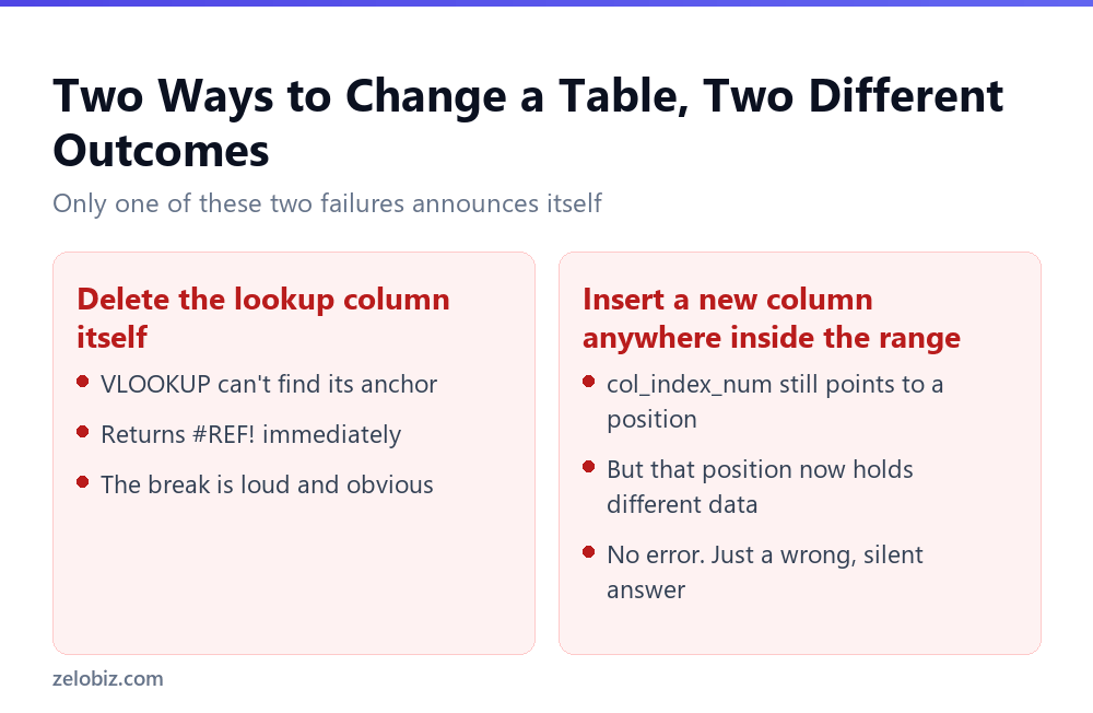
Deleting the lookup column itself breaks VLOOKUP loudly. The formula can’t find its anchor, so Excel throws a #REF! error immediately. You notice right away.

Inserting a column is different. Say col_index_num is 3, pointing to “Price.” Someone inserts a new “Region” column between columns 2 and 3. Excel doesn’t touch the formula. It still says 3. But position 3 in the range is now “Region,” not “Price.”

The formula runs fine. It returns a value. That value just happens to be wrong, and nothing on the screen indicates it. This is the specific failure mode that makes VLOOKUP risky in spreadsheets other people edit, or that get restructured over time.

The Approximate Match Trap

The fourth argument, range_lookup, causes a second, more common mistake. Leave it blank, and Excel defaults to TRUE: an approximate match.

Approximate match assumes the first column of your range is sorted, and returns the closest value at or below your lookup value if no exact one exists. For sorted numeric brackets, like tax tables, that’s exactly what you want. For names, IDs, or product codes, it’s almost never what you want.

Reading VLOOKUP’s Error Codes

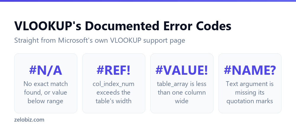
When VLOOKUP does throw an error, the specific code tells you where to look first.

#N/A is the one worth trusting least at face value. It can mean the value truly isn’t there, or it can mean the value exists but has a trailing space, a hidden character, or is stored as text when the lookup value is a number. Same error code, different fix.

A Worked Example

Say column A holds employee IDs, column B holds names, and column C holds department. A lookup formula in another sheet reads =VLOOKUP(A2, Sheet1!A:C, 3, FALSE) to pull each department.

Someone later inserts a “Start Date” column between B and C, to track tenure. Column C is now “Start Date.” Column D is “Department.” The formula still says 3. It now returns a date where a department name used to appear, formatted oddly but not obviously broken at a glance.

This exact scenario, an innocent column insertion months after the original formula was written, is the most common real-world way VLOOKUP quietly goes wrong in shared spreadsheets.

When VLOOKUP Isn’t the Right Tool

VLOOKUP also can’t look to its left. The lookup column must be the first column in table_array, and the return column must sit to its right. If your ID column is to the right of the name you need, VLOOKUP simply can’t reach it without rearranging the sheet.

Two modern alternatives solve both problems at once. INDEX/MATCH references columns by position independently, so an inserted column doesn’t silently shift anything. XLOOKUP goes further, searching in either direction and defaulting to exact match instead of approximate.

Fixing a VLOOKUP That’s Already Gone Wrong

First, find every VLOOKUP formula in the sheet. Press Ctrl+` to toggle formula view, or use Find and Replace to search for “VLOOKUP” in formulas.

Next, check each col_index_num against the current layout. Count the columns in table_array by hand, left to right, and compare that count to what the formula says. A mismatch confirms the problem.

Then update the number to match the new layout. But that’s only a patch. The next person who inserts a column will break it again, in the exact same way.

So for a sheet that gets edited often, a one-time fix isn’t really a fix. It buys time, not safety.

A Habit That Prevents This Entirely

Two changes remove the risk for good. Neither requires learning a new function.

First, convert the data range into an Excel Table, using Insert then Table. Tables use column names in formulas instead of raw cell ranges, so a formula referencing a named column keeps working even after columns shift around it.

Second, switch the lookup itself to INDEX/MATCH. Because it locates the return column by matching a header name rather than counting a fixed number, an inserted column can’t silently point it at the wrong place. That’s covered in full detail in why INDEX/MATCH survives an inserted column.

Why This Mistake Is So Common

Spreadsheets rarely stay static. Someone adds a column for a new metric. Someone else reorders fields to match a report template. Neither person is thinking about a VLOOKUP formula sitting three tabs away.

And that’s exactly the point. The person who breaks the formula usually has no idea it exists. They’re not making a lookup mistake. They’re just editing their own sheet.

So the fix isn’t really about writing VLOOKUP more carefully. It’s about building formulas that survive normal, everyday edits from people who don’t know those formulas are there.

How to Catch This Before It Ships

So how do you catch a shifted VLOOKUP before it reaches a report or a client? A few habits help. None of them are complicated.

First, add a helper column that shows the header name at col_index_num, using INDEX(table_array, 1, col_index_num). If that header ever stops matching what you expect, you know the formula drifted.

Second, use Excel’s own Trace Precedents tool, found on the Formulas tab. It draws an arrow from the formula to the cells it actually reads. A quick glance often shows whether the arrow still points where it should.

Third, and simplest: whenever someone tells you they inserted a column, treat that as a cue to re-check every VLOOKUP nearby. Because the formula itself won’t warn you. Only a manual check will.

What Excel Won’t Tell You

Excel has no built-in alert for this. There’s no warning icon, no flagged cell, no audit trail showing that col_index_num used to mean something else.

That’s worth sitting with for a moment. Excel actively checks for other kinds of problems. It flags text stored as numbers. It flags formulas that reference an empty cell. But a col_index_num that quietly points somewhere new triggers nothing at all, because as far as Excel is concerned, nothing is wrong. The formula ran. It returned a value. That’s a success by Excel’s own definition.

So the responsibility sits entirely with whoever built the formula, or whoever reviews the sheet later. That’s an uncomfortable amount of trust to place in one typed number, especially on a file more than one person touches.

Still, this isn’t a reason to avoid VLOOKUP altogether. It’s a reason to know exactly when its risk is worth accepting, and when it isn’t.

A Quick Self-Check for Any Old Workbook

So if you’ve inherited a spreadsheet full of VLOOKUP formulas, a quick self-check helps before you trust any of them.

First, open each formula and read the col_index_num out loud. Then count the actual columns in table_array yourself, left to right. If the two numbers don’t line up with what the formula is supposed to return, something has already shifted.

Second, spot-check a few results against the source data directly. Because a wrong value often still looks like a reasonable value, this step catches errors a glance at the formula alone won’t.

Third, ask whoever maintains the sheet whether columns were added recently. Often, they’ll remember the exact change, even if they never connected it to a lookup formula elsewhere.

And finally, if the workbook gets edited often by more than one person, treat this as a recurring check, not a one-time fix. Because the same mistake can happen again the very next time someone inserts a column.

Does This Happen With Rows Too?

So far, every example has been about columns, because col_index_num is a column count. But what about inserting a row instead?

Inserting a row is much safer. VLOOKUP’s table_array typically references whole columns or a range that Excel automatically extends, so a new row usually gets absorbed into the existing range without shifting anything.

The one exception is a formula written against a hard-coded, exact range like A2:C50 instead of A:C or a Table. Insert a row past row 50, and that data falls outside the range entirely, causing a genuine, visible miss rather than a silent wrong answer.

Common Questions

The Short Version

So the next time a VLOOKUP formula returns a number that looks slightly off, don’t assume the data is wrong. Check the formula’s col_index_num first. More often than not, that’s exactly where the real problem is hiding.

Putting It All Together

So here’s the whole picture in a few short lines. VLOOKUP counts columns by number, not by name.

Because of that, an inserted column shifts the data without changing the count. So the formula keeps running. But it now points at the wrong spot.

And that’s the part that catches people off guard. There’s no error. No warning. Just a quiet, wrong number sitting where a right one used to be.

So check col_index_num after any column change. Also, type FALSE for exact matches on names or IDs. And for a sheet many people touch, move to INDEX/MATCH.

Because that one habit removes the entire risk, not just for today, but for every edit still to come.